中心極限定理

從這里開始直到高斯分布課程結尾的內容皆為選修部分。

這一部分介紹了高斯分布的由來。如果你想深入學習高斯分布背后的理論，那么請繼續。如果你不想，也可以直接跳到機器人定位課程。

 

什么是中心極限定理？

中心極限定理相當有趣。它說明了如果你從總體中選取足夠多的樣本，並計算這些樣本的均值，這些均值將呈正態分布。只要樣本數量足夠多，並且問題中的變量是獨立和隨機的，那么這條定理便能成立。

這聽起來也許有些理論化了。因此在本堂課的下一部分，我們將會使用 Python 來為你說明這條定理。

 

總體

總體中包含了數據集中的所有值。在這一課中，我們將用到的數據就像下面這樣：

 

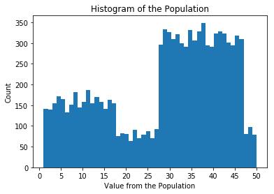
Population Distribution

 

例如，值 15 在總體中大概出現了 160 次，值 50 在總體中大概出現了 70 次。這個總體中一共有 10,000 個數據點。

隨機從這一分布中抽取 100 個數據點，並將這 100 個數據點稱為一個樣本。接着計算該樣本的均值。如果你照此方法反復抽取樣本，得到的均值將呈高斯分布。

隨着大量樣本均值的計算，看着人口分布逐漸向高斯分布靠近，這是一件十分神奇的事。

在本課程的下一部分，我們將為你呈現如何使用 Python 代碼做到這一點。

在本節中，我們將向你介紹如何運用中心極限定理。我們將：

• 從總體中生成隨機樣本
• 獲取樣本均值
• 將結果均值可視化

你會看到，雖然總體不遵循高斯分布，但樣本均值的結果分布確實看起來符合高斯分布。

要開始整個任務，請運行下面的代碼單元格。這個單元格將通過運行一個輔助函數來創建總體數據，然后將總體數據可視化，並計算總體數據的平均值。總人口中有10,000個數據點。

如果多次運行該單元格，你會發現分布稍有變化；但是，總體形狀保持不變。

import helpers
import numpy as np
%matplotlib inline

population_data = helpers.distribution(50, 10000, 100)
helpers.histogram_visualization(population_data)
print('population mean ', np.mean(population_data))

　　

從人口中抽樣

下一個代碼單元格將隨機從總體中選擇N個數據點。這N個數據點將被稱為樣本。我們使用numpy庫的random.choice方法隨機選擇N個值，你可以在 這里 讀取這些值。

運行下面的代碼單元格，查看一些示例輸出。該代碼從總體中隨機抽取10個數據點，制作一個大小為10的樣本。

def random_sample(population_data, sample_size):
    return np.random.choice(population_data, size = sample_size)

random_sample(population_data, 10)

array([33, 40, 29, 13, 48,  7, 41, 11, 32,  1])

計算樣本均值

接下來我們將使用numpy庫來計算每個隨機生成的樣本的平均值。

def sample_mean(sample):
    return np.mean(sample)

# take a sample from the population
example_sample = random_sample(population_data, 10)

# calculate the mean of the sample and output the results
sample_mean(example_sample)　

29.300000000000001

中心極限定理結果

現在，我們將使用random_sample（）函數和sample_mean（）函數來演示中心極限定理是如何運用的。

下面的代碼包含一個for循環，該循環會制作一個大小為N的隨機樣本，然后取樣本的均值，並將該均值存儲在列表中。 for循環的每次迭代都會有一個不同的隨機樣本。研究下面的代碼，然后運行該單元格。

###
# Code for showing how the central limit theorem works.
# The function inputs:
# population - population data
# n - sample size
# iterations - number of times to draw random samples

def central_limit_theorem(population, n, iterations):
    sample_means_results = []
    for i in range(iterations):
        # get a random sample from the population of size n
        sample = random_sample(population, n)
        
        # calculate the mean of the random sample 
        # and append the mean to the results list
        sample_means_results.append(sample_mean(sample))
    return sample_means_results

print('Means of all the samples ')
central_limit_theorem(population_data, 10, 10000)

　　

[25.600000000000001,
 22.800000000000001,
 30.0,
 28.899999999999999,
 32.200000000000003,
 29.399999999999999,
 32.0,
 35.299999999999997,
 25.600000000000001,

35.5,
 31.300000000000001,
 24.5,
 28.300000000000001,
 23.300000000000001,
 ...]

將結果可視化 —— 樣本容量= 30

下一個單元格將計算每個大小為30的一萬個樣本的均值，然后使用直方圖將樣本均值可視化。需要注意的是，這個可視化結果大致與高斯分布類似。

import matplotlib.pyplot as plt

def visualize_results(sample_means):

plt.hist(sample_means, bins = 30)
plt.title('Histogram of the Sample Means')
plt.xlabel('Mean Value')
plt.ylabel('Count')

# Take random sample and calculate the means
sample_means_results = central_limit_theorem(population_data, 30, 10000)

# Visualize the results
visualize_results(sample_means_results)

　　

所以我們剛開始使用的人口樣本肯定不符合高斯分布。但是，通過對分布樣本進行抽樣並計算樣本均值，我們最終會看到一些看起來像高斯分布的東西。

將結果可視化 —— 樣本容量= 1

根據中心極限定理，樣本容量需要足夠大。一般的經驗法則是樣本容量應該大於或等於30。讓我們嘗試使用不同的樣本容量來查看會有什么不同的結果。

一個比較誇張的情況是樣本容量為1。它的分布應該與原始人口的分布類似。運行下面的代碼，查看結果。

# Take random sample and calculate the means
sample_means_results = central_limit_theorem(population_data, 1, 10000)

# Visualize the results
visualize_results(sample_means_results)

　　

將結果可視化 ——樣本容量= 10

現在，我們使用建議的最小樣本容量，即30，看看會發生什么。

# Take random sample and calculate the means
sample_means_results = central_limit_theorem(population_data, 10, 10000)

# Visualize the results
visualize_results(sample_means_results)

　　

樣本容量為10時，樣本均值的分布看起來類似高斯分布。

將結果可視化 —— 樣本容量= 1000

讓我們繼續嘗試，並使用更大的樣本容量：這次為1000。

# Take random sample and calculate the means
sample_means_results = central_limit_theorem(population_data, 1000, 10000)

# Visualize the results
visualize_results(sample_means_results)

　　

將結果可視化 —— 樣本容量= 10000

如果樣本容量等於人口數量，會發生什么情況？因為我們隨機抽樣進行替換，所以其中一個樣本不太可能是完全的人口數據；然而，由於每個樣本可能與人口相似，因此標准差應該進一步降低。

# Take random sample and calculate the means
sample_means_results = central_limit_theorem(population_data, 10000, 10000)

# Visualize the results
visualize_results(sample_means_results)

　　

結論

我們還要注意，這些分布的中心接近原始人口均值。

想一想是否要收集現實世界中的數據。如果你想找到世界各地人口的身高分布，你可以測量每個人的身高並分析結果。如果使用該結果的均值，那么你將獲得真實的人體高度平均值；然而，要使用這個辦法去衡量整個世界人口是不可行的。

相反，你可以使用身高的一個樣本。如果只測量了三十人，你的抽樣均值可能會與人口平均值相差較大。但是，如果測量了20億個隨機選擇的人，那么樣本均值可能更接近人口均值。你的樣本越大，樣本均值就越可能與真實的人口均值相匹配。