在初始概念篇中,我們簡單提到了時間序列由趨勢、周期性、季節性、誤差構成,本文將介紹如何將時間序列的這些成分分解出來。分解的使用場景有很多,比如當我們需要計算該時間序列是否具有季節性,或者我們要去除該時間序列的趨勢和季節性,讓時間序列變得平穩時都會用到時間序列分解。
加法和乘法時間序列
時間序列的各個觀測值可以是以上成分相加或相乘得到:
Value = Trend + Seasonality + Error
Value = Trend * Seasonality * Error
分解
下面的代碼展示了如何用python從時間序列中分解出相應的成分:
from statsmodels.tsa.seasonal import seasonal_decompose
from dateutil.parser import parse

# Import Data
df = pd.read_csv('https://raw.githubusercontent.com/selva86/datasets/master/a10.csv', parse_dates=['date'], index_col='date')

# Multiplicative Decomposition
result_mul = seasonal_decompose(df['value'], model='multiplicative', extrapolate_trend='freq')

# Additive Decomposition
result_add = seasonal_decompose(df['value'], model='additive', extrapolate_trend='freq')

# Plot
plt.rcParams.update({'figure.figsize': (10,10)})
result_mul.plot().suptitle('Multiplicative Decompose', fontsize=22)
result_add.plot().suptitle('Additive Decompose', fontsize=22)
plt.show()

# Extract the Components ----# Actual Values = Product of (Seasonal * Trend * Resid)
df_reconstructed = pd.concat([result_mul.seasonal, result_mul.trend, result_mul.resid, result_mul.observed], axis=1)
df_reconstructed.columns = ['seas', 'trend', 'resid', 'actual_values']
df_reconstructed.head()
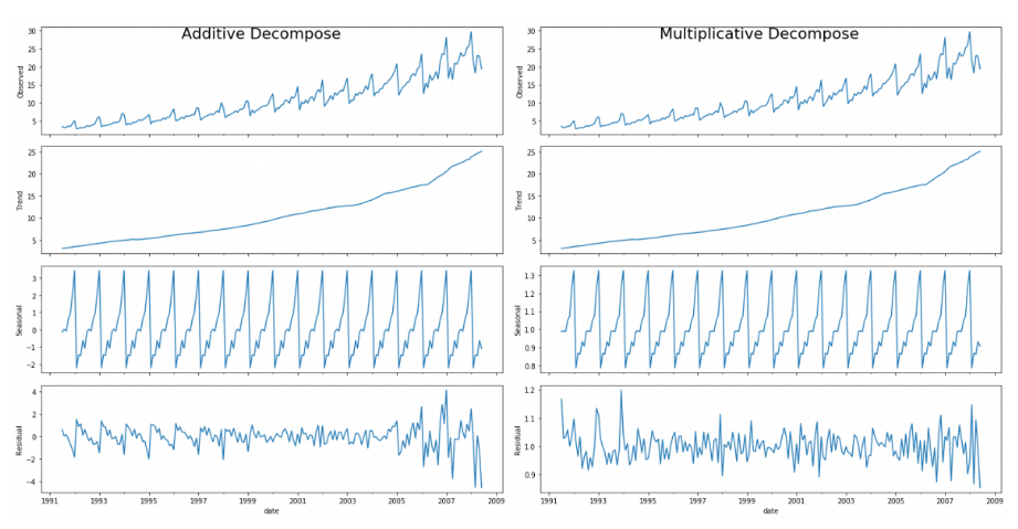
對比上面的加法分解和乘法分解可以看到,加法分解的殘差圖中有一些季節性成分沒有被分解出去,而乘法相對而言隨機多了(越隨機意味着留有的成分越少),所以對於當前時間序列來說,乘法分解更適合。
小結
時間序列分解不僅可以讓我們更清晰的了解序列的特性,有時候人們還會用分解出的殘差序列(誤差)代替原始序列來做預測,因為原始時間序列一般是非平穩序列,而這個殘差序列是平穩序列,有助於我們做出更好的預測,當然預測后的序列還要加回或乘回趨勢成分和季節性成分,平穩序列的具體內容將在下一篇文章中介紹。
ok,本篇就這么多內容啦~,感謝閱讀O(∩_∩)O。