用python做時間序列預測九：ARIMA模型簡介

本篇介紹時間序列預測常用的ARIMA模型，通過了解本篇內容，將可以使用ARIMA預測一個時間序列。

什么是ARIMA？

• ARIMA是'Auto Regressive Integrated Moving Average'的簡稱。
• ARIMA是一種基於時間序列歷史值和歷史值上的預測誤差來對當前做預測的模型。
• ARIMA整合了自回歸項AR和滑動平均項MA。
• ARIMA可以建模任何存在一定規律的非季節性時間序列。
• 如果時間序列具有季節性，則需要使用SARIMA(Seasonal ARIMA)建模，后續會介紹。

ARIMA模型參數

ARIMA模型有三個超參數：p,d,q

• p
  AR(自回歸)項的階數。需要事先設定好，表示y的當前值和前p個歷史值有關。

• d
  使序列平穩的最小差分階數，一般是1階。非平穩序列可以通過差分來得到平穩序列，但是過度的差分，會導致時間序列失去自相關性，從而失去使用AR項的條件。

• q
  MA(滑動平均)項的階數。需要事先設定好，表示y的當前值和前q個歷史值AR預測誤差有關。實際是用歷史值上的AR項預測誤差來建立一個類似歸回的模型。

ARIMA模型表示

• AR項表示
  一個p階的自回歸模型可以表示如下：
  
  c是常數項，εt是隨機誤差項。
  對於一個AR(1)模型而言：
  當 ϕ1=0 時,yt 相當於白噪聲；
  當 ϕ1=1 並且 c=0 時,yt 相當於隨機游走模型；
  當 ϕ1=1 並且 c≠0 時,yt 相當於帶漂移的隨機游走模型；
  當 ϕ1<0 時,yt 傾向於在正負值之間上下浮動。

• MA項表示
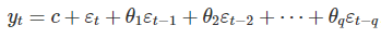
  一個q階的預測誤差回歸模型可以表示如下：
  
  c是常數項，εt是隨機誤差項。
  yt 可以看成是歷史預測誤差的加權移動平均值，q指定了歷史預測誤差的期數。

• 完整表示
  
  即: 被預測變量Yt = 常數+Y的p階滯后的線性組合 + 預測誤差的q階滯后的線性組合

ARIMA模型定階

看圖定階

差分階數d

• 如果時間序列本身就是平穩的，就不需要差分，所以此時d=0。
• 如果時間序列不平穩，那么主要是看時間序列的acf圖，如果acf表現為10階或以上的拖尾，那么需要進一步的差分，如果acf表現為1階截尾，則可能是過度差分了，最好的差分階數是使acf先拖尾幾階，然后截尾。
• 有的時候，可能在2個階數之間無法確定用哪個，因為acf的表現差不多，那么就選擇標准差小的序列。
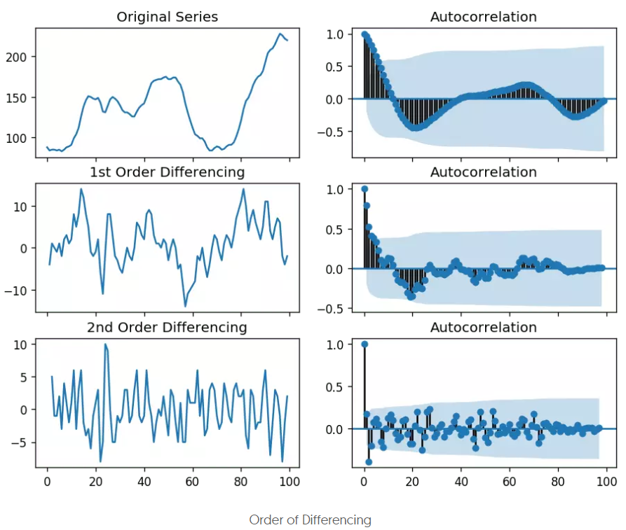
• 下面是原時間序列、一階差分后、二階差分后的acf圖：
  
  可以看到，原序列的acf圖的拖尾階數過高了，而二階差分后的截尾階數過小了，所以一階差分更合適。

python代碼：

import numpy as np, pandas as pd
from statsmodels.graphics.tsaplots import plot_acf, plot_pacf
import matplotlib.pyplot as plt
plt.rcParams.update({'figure.figsize':(9,7), 'figure.dpi':120})

# Import data : Internet Usage per Minute
df = pd.read_csv('https://raw.githubusercontent.com/selva86/datasets/master/wwwusage.csv', names=['value'], header=0)

# Original Series
fig, axes = plt.subplots(3, 2, sharex=True)
axes[0, 0].plot(df.value); axes[0, 0].set_title('Original Series')
plot_acf(df.value, ax=axes[0, 1])

# 1st Differencing
axes[1, 0].plot(df.value.diff()); axes[1, 0].set_title('1st Order Differencing')
plot_acf(df.value.diff().dropna(), ax=axes[1, 1])

# 2nd Differencing
axes[2, 0].plot(df.value.diff().diff()); axes[2, 0].set_title('2nd Order Differencing')
plot_acf(df.value.diff().diff().dropna(), ax=axes[2, 1])

plt.show()

AR階數p

AR的階數p可以通過pacf圖來設定，因為AR各項的系數就代表了各項自變量x對因變量y的偏自相關性。

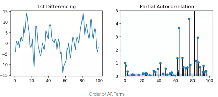
可以看到，lag1，lag2之后，偏自相關落入了藍色背景區間內，表示不相關，所以這里階數可以選擇2，或者保守點選擇1。

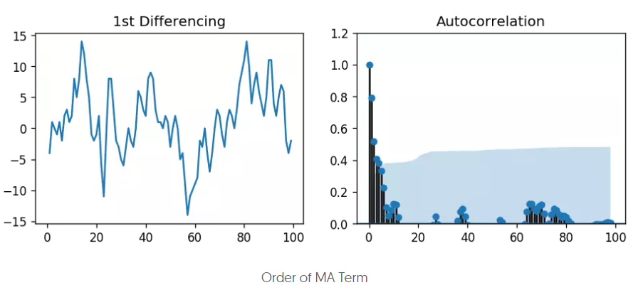
MA階數q

MA階數通過acf圖來設定，因為MA是預測誤差，預測誤差是自回歸預測和真實值之間的偏差。定階過程類似AR階數的設定過程。這里可以選擇3，或者保守點選擇2。

信息准則定階

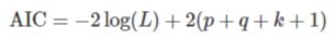
• AIC(Akaike Information Criterion)
  
  L是數據的似然函數，k=1表示模型考慮常數c，k=0表示不考慮。最后一個1表示算上誤差項，所以其實第二項就是2乘以參數個數。

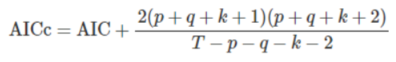
• AICc（修正過的AIC）
  

• BIC(Bayesian Information Criterion)
  

注意事項：

• 信息准則越小，說明參數的選擇越好，一般使用AICc或者BIC。
• 差分d，不要使用信息准則來判斷，因為差分會改變了似然函數使用的數據，使得信息准則的比較失去意義，所以通常用別的方法先選擇出合適的d。
• 信息准則的好處是可以在用模型給出預測之前，就對模型的超參做一個量化評估，這對批量預測的場景尤其有用，因為批量預測往往需要在程序執行過程中自動定階。

構建ARIMA模型

from statsmodels.tsa.arima_model import ARIMA

# 1,1,2 ARIMA Model
model = ARIMA(df.value, order=(1,1,2))
model_fit = model.fit(disp=0)
print(model_fit.summary())

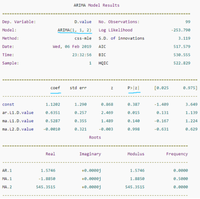
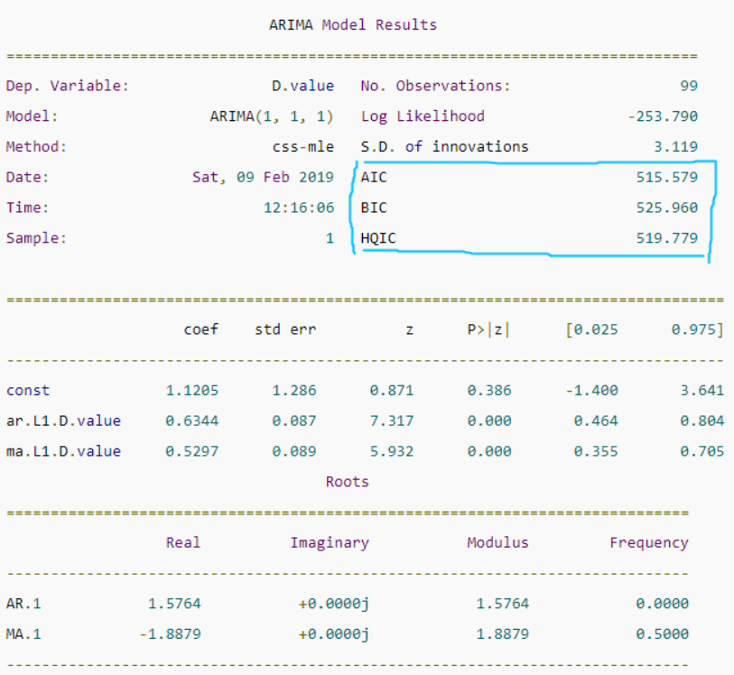
中間的表格列出了訓練得到的模型各項和對應的系數，如果系數很小，且‘P>|z|’ 列下的P-Value值遠大於0.05，則該項應該去掉，比如上圖中的ma部分的第二項，系數是-0.0010,P-Value值是0.998,那么可以重建模型為ARIMA(1,1,1)，從下圖可以看到，修改階數后的模型的AIC等信息准則都有所降低：

檢查殘差

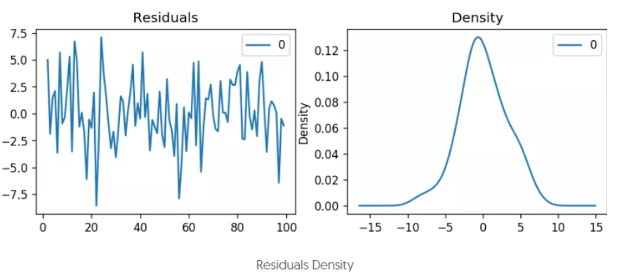
通常會檢查模型擬合的殘差序列，即訓練數據原本的序列減去訓練數據上的擬合序列后的序列。該序列越符合隨機誤差分布(均值為0的正態分布)，說明模型擬合的越好，否則，說明還有一些因素模型未能考慮。

• python實現：

# Plot residual errors
residuals = pd.DataFrame(model_fit.resid)
fig, ax = plt.subplots(1,2)
residuals.plot(title="Residuals", ax=ax[0])
residuals.plot(kind='kde', title='Density', ax=ax[1])
plt.show()

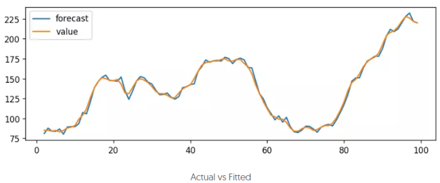
模型擬合

# Actual vs Fitted
model_fit.plot_predict(dynamic=False)
plt.show()

模型預測

除了在訓練數據上擬合，一般都會預留一部分時間段作為模型的驗證，這部分時間段的數據不參與模型的訓練。

from statsmodels.tsa.stattools import acf

# Create Training and Test
train = df.value[:85]
test = df.value[85:]

# Build Model
# model = ARIMA(train, order=(3,2,1))  
model = ARIMA(train, order=(1, 1, 1))  
fitted = model.fit(disp=-1)  

# Forecast
fc, se, conf = fitted.forecast(15, alpha=0.05)  # 95% conf

# Make as pandas series
fc_series = pd.Series(fc, index=test.index)
lower_series = pd.Series(conf[:, 0], index=test.index)
upper_series = pd.Series(conf[:, 1], index=test.index)

# Plot
plt.figure(figsize=(12,5), dpi=100)
plt.plot(train, label='training')
plt.plot(test, label='actual')
plt.plot(fc_series, label='forecast')
plt.fill_between(lower_series.index, lower_series, upper_series, 
                 color='k', alpha=.15)
plt.title('Forecast vs Actuals')
plt.legend(loc='upper left', fontsize=8)
plt.show()

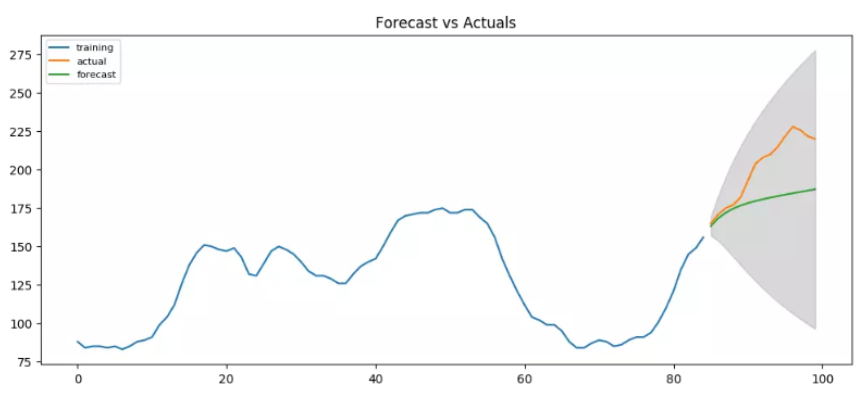
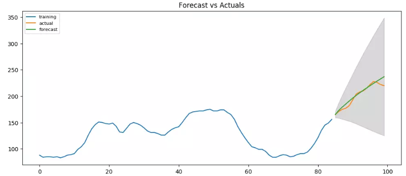
這是在ARIMA(1,1,1)下的預測結果，給出了一定的序列變化方向，看上去還是可以的。不過所有的預測值，都在真實值以下，所以還可以試試看有沒有別的更好的階數組合。
其實如果嘗試用ARIMA(3,2,1)會發現預測的更好：

AUTO ARIMA

通過預測結果來推斷模型階數的好壞畢竟還是耗時耗力了些，一般可以通過計算AIC或BIC的方式來找出更好的階數組合。pmdarima模塊的auto_arima方法就可以讓我們指定一個階數上限和信息准則計算方法，從而找到信息准則最小的階數組合。

from statsmodels.tsa.arima_model import ARIMA
import pmdarima as pm

df = pd.read_csv('https://raw.githubusercontent.com/selva86/datasets/master/wwwusage.csv', names=['value'], header=0)

model = pm.auto_arima(df.value, start_p=1, start_q=1,
                      information_criterion='aic',
                      test='adf',       # use adftest to find optimal 'd'
                      max_p=3, max_q=3, # maximum p and q
                      m=1,              # frequency of series
                      d=None,           # let model determine 'd'
                      seasonal=False,   # No Seasonality
                      start_P=0, 
                      D=0, 
                      trace=True,
                      error_action='ignore',  
                      suppress_warnings=True, 
                      stepwise=True)

print(model.summary())

# Forecast
n_periods = 24
fc, confint = model.predict(n_periods=n_periods, return_conf_int=True)
index_of_fc = np.arange(len(df.value), len(df.value)+n_periods)

# make series for plotting purpose
fc_series = pd.Series(fc, index=index_of_fc)
lower_series = pd.Series(confint[:, 0], index=index_of_fc)
upper_series = pd.Series(confint[:, 1], index=index_of_fc)

# Plot
plt.plot(df.value)
plt.plot(fc_series, color='darkgreen')
plt.fill_between(lower_series.index, 
                 lower_series, 
                 upper_series, 
                 color='k', alpha=.15)

plt.title("Final Forecast of WWW Usage")
plt.show()

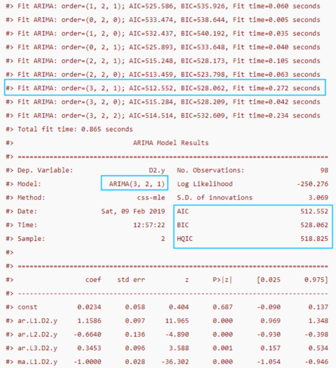
從輸出可以看到，模型采用了ARIMA(3,2,1)的組合來預測，因為該組合計算出的AIC最小。

如何自動構建季節性ARIMA模型？

如果模型帶有季節性，則除了p,d,q以外，模型還需要引入季節性部分：

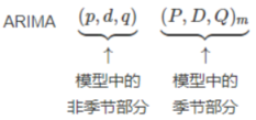
與非季節性模型的區別在於，季節性模型都是以m為固定周期來做計算的，比如D就是季節性差分，是用當前值減去上一個季節周期的值，P和Q和非季節性的p,q的區別也是在於前者是以季節窗口為單位，而后者是連續時間的。
上節介紹的auto arima的代碼中，seasonal參數設為了false，構建季節性模型的時候，把該參數置為True，然后對應的P，D，Q,m參數即可，代碼如下：

# !pip3 install pyramid-arima
import pmdarima as pm
# Seasonal - fit stepwise auto-ARIMA
smodel = pm.auto_arima(data, start_p=1, start_q=1,
                         test='adf',
                         max_p=3, max_q=3, m=12,
                         start_P=0, seasonal=True,
                         d=None, D=1, trace=True,
                         error_action='ignore',  
                         suppress_warnings=True, 
                         stepwise=True)
smodel.summary()

注意這里的stepwise參數，默認值就是True，表示用stepwise algorithm來選擇最佳的參數組合，會比計算所有的參數組合要快很多，而且幾乎不會過擬合，當然也有可能忽略了最優的組合參數。所以如果你想讓模型自動計算所有的參數組合，然后選擇最優的，可以將stepwise設為False。

如何在預測中引入其它相關的變量？

在時間序列模型中，還可以引入其它相關的變量，這些變量稱為exogenous variable(外生變量，或自變量)，比如對於季節性的預測，除了之前說的通過加入季節性參數組合以外，還可以通過ARIMA模型加外生變量來實現，那么這里要加的外生變量自然就是時間序列中的季節性序列了(通過時間序列分解得到)。需要注意的是，對於季節性來說，還是用季節性模型來擬合比較合適，這里用外生變量的方式只是為了方便演示外生變量的用法。因為對於引入了外生變量的時間序列模型來說，在預測未來的值的時候，也要對外生變量進行預測的，而用季節性做外生變量的方便演示之處在於，季節性每期都一樣的，比如年季節性，所以直接復制到3年就可以作為未來3年的季節外生變量序列了。

def load_data():
    """
    航司乘客數時間序列數據集
    該數據集包含了1949-1960年每個月國際航班的乘客總數。
    """
    from datetime import datetime
    date_parse = lambda x: datetime.strptime(x, '%Y-%m-%d')
    data = pd.read_csv('https://www.analyticsvidhya.com/wp-content/uploads/2016/02/AirPassengers.csv', index_col='Month', parse_dates=['Month'], date_parser=date_parse)
    # print(data)
    # print(data.index)
    ts = data['value']
    # print(ts.head(10))
    # plt.plot(ts)
    # plt.show()
    return ts,data

# 加載時間序列數據
_ts,_data = load_data()
# 時間序列分解
result_mul = seasonal_decompose(_ts[-36:],  # 3 years
                                model='multiplicative',
                                freq=12,
                                extrapolate_trend='freq')
_seasonal_frame = result_mul.seasonal[-12:].to_frame()
_seasonal_frame['month'] = pd.to_datetime(_seasonal_frame.index).month
# seasonal_index = result_mul.seasonal[-12:].index
# seasonal_index['month'] = seasonal_index.month.values
print(_seasonal_frame)
_data['month'] = _data.index.month
print(_data)
_df = pd.merge(_data, _seasonal_frame, how='left', on='month')
_df.columns = ['value', 'month', 'seasonal_index']
print(_df)
print(_df.index)
_df.index = _data.index  # reassign the index.
print(_df.index)

build_arima(_df,_seasonal_frame,_data)

# SARIMAX Model
sxmodel = pm.auto_arima(df[['value']],
						exogenous=df[['seasonal_index']],
						start_p=1, start_q=1,
						test='adf',
						max_p=3, max_q=3, m=12,
						start_P=0, seasonal=False,
						d=1, D=1, trace=True,
						error_action='ignore',
						suppress_warnings=True,
						stepwise=True)
sxmodel.summary()
# Forecast
n_periods = 36
fitted, confint = sxmodel.predict(n_periods=n_periods,
								  exogenous=np.tile(seasonal_frame['y'].values, 3).reshape(-1, 1),
								  return_conf_int=True)
index_of_fc = pd.date_range(data.index[-1], periods = n_periods, freq='MS')
# make series for plotting purpose
fitted_series = pd.Series(fitted, index=index_of_fc)
lower_series = pd.Series(confint[:, 0], index=index_of_fc)
upper_series = pd.Series(confint[:, 1], index=index_of_fc)

# Plot
plt.plot(data['y'])
plt.plot(fitted_series, color='darkgreen')
plt.fill_between(lower_series.index,
				 lower_series,
				 upper_series,
				 color='k', alpha=.15)

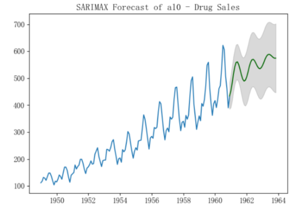
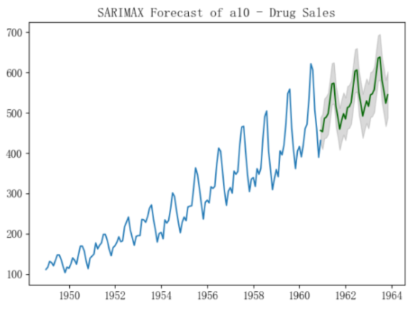
plt.title("SARIMAX Forecast of a10 - Drug Sales")
plt.show()

以下是結果比較:

• 選擇ARIMA(3,1,1)來預測：
  
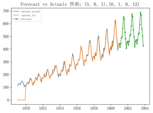
• 選擇季節性模型SARIMA(3,0,1),(0,1,0,12)來預測:
  
• 選擇帶季節性外生變量的ARIMA(3,1,1)來預測:
  

ok,本篇就這么多內容啦~，下一篇將基於一個實際的例子來介紹完整的預測實現過程，感謝閱讀O(∩_∩)O。