Python機器學習（十）經典算法大全

本文轉載自查看原文 2020-06-17 17:57 1008 人工智能之機器學習

1.KNN 分類算法

由於knn算法涉及到距離的概念，KNN 算法需要先進行歸一化處理

1.1 歸一化處理 scaler

from sklearn.preprocessing import StandardScaler

standardScaler =StandardScaler()

standardScaler.fit(X_train)
X_train_standard = standardScaler.transform(X_train)
X_test_standard = standardScaler.transform(X_test)

歸一化之后送入模型進行訓練

from sklearn.neighbors import KNeighborsClassifier

knn_clf = KNeighborsClassifier(n_neighbors=8)
knn_classifier.fit(X_train_standard, y_train)
y_predict = knn_clf.predict(X_test_standard)

# 默認的預測指標為分類准確度
knn_clf.score(X_test, y_test)

1.2 網格搜索 GridSearchCV

使用網格搜索來確定KNN算法合適的超參數

from sklearn.model_selection import GridSearchCV

param_grid = [
    {
        ‘weights‘:[‘uniform‘],
        ‘n_neighbors‘:[ i for i in range(1, 11)]
    },
    {
        ‘weights‘:[‘distance‘],
        ‘n_neighbors‘:[i for i in range(1, 11)],
        ‘p‘:[p for p in range(1, 6)]
    }
]

grid_search = GridSearchCV(knn_clf, param_grid, n_jobs=-1, verbose=2)
grid_search.fit(X_train_standard, y_train)
knn_clf = grid_search.best_estimator_
knn_clf.score(X_test_standard, y_test)

1.3 交叉驗證

GridSearchCV 本身就包括了交叉驗證，也可自己指定參數cv

默認GridSearchCV的KFold平分為3份
自己指定交叉驗證，查看交叉驗證成績
```
from sklearn.model_selection import cross_val_score

# 默認為分成3份
cross_val_score(knn_clf, X_train, y_train, cv=5)
```
這里默認的scoring標准為 accuracy

有許多可選的參數，具體查看官方文檔
封裝成函數，在fit完模型之后，一次性查看多個評價指標的成績

這里選的只是針對分類算法的指標，也可以是針對回歸，聚類算法的評價指標

def cv_score_train_test(model):
    num_cv = 5
    score_list = ["accuracy","f1", "neg_log_loss", "roc_auc"]
    for score in score_list:
        print(score,"\t train:",cross_val_score(model, X_train, y_train, cv=num_cv, scoring=score).mean())
        print(score,"\t test:",cross_val_score(model, X_test, y_test, cv=num_cv, scoring=score).mean())

2. 線性回歸

2.1 簡單線性回歸

from sklearn.linear_model import LinearRegression

linreg = LinearRegression()

linreg.fit(X_train, y_train)
#查看截距和系數

print linreg.intercept_
print linreg.coef_
lin_reg.score(X_test, y_test)

y_predict = linreg.predict(X_test)

2.2 多元線性回歸

在更高維度的空間中的“直線”，即數據不只有一個維度，而具有多個維度

代碼和上面的簡單線性回歸相同

3. 梯度下降法

使用梯度下降法之前，需要對數據進行歸一化處理

3.1 隨機梯度下降線性回歸

SGD_reg

from sklearn.linear_model import SGDRegressor

sgd_reg = SGDRegressor(max_iter=100)
sgd_reg.fit(X_train_standard, y_train_boston)
sgd_reg.score(X_test_standard, y_test_boston)

3.2 確定梯度下降計算的准確性

以多元線性回歸的目標函數（損失函數）為例

比較使用數學推導式（得出具體解析解）的方法和debug的近似方法的比較

# 編寫損失函數
def J(theta, X_b, y):
    try:
        return np.sum((y - X_b.dot(theta)) ** 2) / len(y)
    except:
        return float(‘inf‘)
        
# 編寫梯度函數（使用數學推導方式得到的）
def dJ_math(theta, X_b, y):
    return X_b.T.dot(X_b.dot(theta) - y) * 2.0 / len(y)
    
# 編寫梯度函數（用來debug的形式）
def dJ_debug(theta, X_b, y, epsilon=0.01):
    res = np.empty(len(theta))
    for i in range(len(theta)):
        theta_1 = theta.copy()
        theta_1[i] += epsilon
        theta_2 = theta.copy()
        theta_2[i] -= epsilon
        res[i] = (J(theta_1, X_b, y) - J(theta_2, X_b, y)) / (2 * epsilon)
    return res

# 批量梯度下降，尋找最優的theta
def gradient_descent(dJ, X_b, y, initial_theta, eta, n_iters=1e4, epsilon=1e-8):
    theta = initial_theta
    i_iter = 0
    
    while i_iter < n_iters:
        gradient = dJ(theta, X_b, y)
        last_theta = theta
        theta = theta - eta * gradient
        
        if(abs(J(theta, X_b, y) - J(last_theta, X_b, y)) < epsilon):
            break
        
        i_iter += 1
    return theta

# 函數入口參數第一個，要指定dJ函數是什么樣的
X_b = np.hstack([np.ones((len(X), 1)), X])
initial_theta = np.zeros(X_b.shape[1])
eta = 0.01

# 使用debug方式
theta = gradient_descent(dJ_debug, X_b, y, initial_theta, eta)
# 使用數學推導方式
theta = gradient_descent(dJ_math, X_b, y, initial_theta, eta)
# 得出的這兩個theta應該是相同的

4. PCA算法

由於是求方差最大，因此使用的是梯度上升法

PCA算法不能在前處理進行歸一化處理，否則將會找不到主成分

4.1 代碼流程

# 對於二維的數據樣本來說
from sklearn.decomposition import PCA

pca = PCA(n_components=1) #指定需要保留的前n個主成分，不指定為默認保留所有
pca.fit(X)

比如，要使用KNN分類算法，先進行數據的降維操作

from sklearn.decomposition import PCA

pca = PCA(n_components=2)  #這里也可以給一個百分比，代表想要保留的數據的方差占比
pca.fit(X_train)

#訓練集和測試集需要進行相同降維處理操作
X_train_reduction = pca.transform(X_train)
X_test_reduction = pca.transform(X_test)

#降維完成后就可以送給模型進行擬合
knn_clf = KNeighborsClassifier()
knn_clf.fit(X_train_reduction, y_train)
knn_clf.score(X_test_reduction, y_test)

4.2 降維的維數和精度的取舍

指定的維數，能解釋原數據的方差的比例

pca.explained_variance_ratio_

# 指定保留所有的主成分
pca = PCA(n_components=X_train.shape[1])
pca.fit(X_train)
pca.explained_variance_ratio_

# 查看降維后特征的維數
pca.n_components_

把數據降維到2維，可以進行scatter的可視化操作

4.3 PCA數據降噪

先使用pca降維，之后再反向，升維

from sklearn.decomposition import PCA

pca = PCA(0.7)
pca.fit(X)
pca.n_components_

X_reduction = pca.transform(X)
X_inversed = pca.inverse_transform(X_reduction)

5. 多項式回歸與模型泛化

多項式回顧需要指定最高的階數， degree

擬合的將不再是一條直線

只有一個特征的樣本，進行多項式回歸可以擬合出曲線，並且在二維平面圖上進行繪制
而對於具有多個特征的樣本，同樣可以進行多項式回歸，但是不能可視化擬合出來的曲線

5.1 多項式回歸和Pipeline

from sklearn.preprocessing import PolynomialFeatures
from sklearn.linear_model import LinearRegression
from sklearn.preprocessing import StandardScaler
from sklearn.pipeline import Pipeline


poly_reg = Pipeline([
    ("poly", PolynomialFeatures(degree=2)),
    ("std_scaler", StandardScaler()),
    ("lin_reg", LinearRegression())
])

poly_reg.fit(X, y)
y_predict = poly_reg.predict(X)

# 對二維數據點可以繪制擬合后的圖像
plt.scatter(X, y)
plt.plot(np.sort(x), y_predict[np.argsort(x)], color=‘r‘)
plt.show()
#更常用的是，把pipeline寫在函數中
def PolynomialRegression(degree):
    return Pipeline([
        ("poly", PolynomialFeatures(degree=degree)),
        ("std_scaler", StandardScaler()),
        ("lin_reg", LinearRegression())
    ])

poly2_reg = PolynomialRegression(degree=2)
poly2_reg.fit(X, y)

y2_predict = poly2_reg.predict(X)
mean_squared_error(y, y2_predict)

5.2 GridSearchCV 和 Pipeline

明確：

GridSearchCV：用於尋找給定模型的最優的參數
Pipeline：用於將幾個流程整合在一起（PolynomialFeatures()、StandardScaler()、LinearRegression()）

如果非要把上兩者寫在一起，應該把指定好param_grid參數的grid_search作為成員，傳遞給Pipeline

5.3 模型泛化之嶺回歸（Ridge）

首先明確：

模型泛化是為了解決模型過擬合的問題
嶺回歸是模型正則化的一種處理方式，也稱為L2正則化
嶺回歸是線性回歸的一種正則化處理后的模型（作為pipeline的成員使用）

from sklearn.linear_model import Ridge
from sklearn.preprocessing import PolynomialFeatures
from sklearn.preprocessing import StandardScaler
from sklearn.pipeline import Pipeline

def RidgeRegression(degree, alpha):
    return Pipeline([
        ("poly", PolynomialFeatures(degree=degree)),
        ("std_scaler", StandardScaler()),
        ("ridge_reg", Ridge(alpha=alpha))
    ])

ridge_reg = RidgeRegression(degree=20, alpha=0.0001)
ridge_reg.fit(X_train, y_train)

y_predict = ridge_reg.predict(X_test)
mean_squared_error(y_test, y_predict)

代碼中：

alpha為L2正則項前面的系數，代表的含義與LASSO回歸相同

alpha越小，越傾向於選擇復雜模型
alpha越大，越傾向於選擇簡單模型

Ridge回歸、LASSO回歸的區別

Ridge：更傾向於保持為曲線
LASSO：更傾向於變為直線（即趨向於使得部分theta變成0，因此有特征選擇的作用）

5.4 模型泛化之LASSO回歸

嶺回歸是模型正則化的一種處理方式，也稱為L1正則化
嶺回歸是線性回歸的一種正則化處理后的模型（作為pipeline的成員使用）

from sklearn.linear_model import Lasso
from sklearn.preprocessing import PolynomialFeatures
from sklearn.preprocessing import StandardScaler
from sklearn.pipeline import Pipeline

def LassoRegression(degree, alpha):
    return Pipeline([
        ("poly", PolynomialFeatures(degree=degree)),
        ("std_scaler", StandardScaler()),
        ("lasso_reg", Lasso(alpha=alpha))
    ])

lasso_reg = LassoRegression(3, 0.01)
lasso_reg.fit(X_train, y_train)

y_predict = lasso_reg.predict(X_test)
mean_squared_error(y_test, y_predict)

6. 邏輯回歸

將樣本特征與樣本發生的概率聯系起來。

既可看做回歸算法，也可分類算法
通常作為二分類算法

6.1 繪制決策邊界

# 不規則決策邊界繪制方法
def plot_decision_boundary(model, axis):

    x0, x1 = np.meshgrid(
        np.linspace(axis[0], axis[1], int((axis[1] - axis[0]) * 100)).reshape(-1, 1),
        np.linspace(axis[2], axis[3], int((axis[3] - axis[2]) * 100)).reshape(-1, 1)
    )
    X_new = np.c_[x0.ravel(), x1.ravel()]

    y_predict = model.predict(X_new)
    zz = y_predict.reshape(x0.shape)

    from matplotlib.colors import ListedColormap
    custom_cmap = ListedColormap([‘#EF9A9A‘, ‘#FFF59D‘, ‘#90CAF9‘])

    plt.contourf(x0, x1, zz, linewidth=5, cmap=custom_cmap)
    
    
#此處為線性邏輯回歸
from sklearn.linear_model import LogisticRegression
log_reg = LogisticRegression()
log_reg.fit(X_train, y_train)
log_reg.score(X_test, y_test)
繪制決策邊界

plot_decision_boundary(log_reg, axis=[4, 7.5, 1.5, 4.5])
plt.scatter(X[y==0, 0], X[y==0, 1], color=‘r‘)
plt.scatter(X[y==1, 0], X[y==1, 1], color=‘blue‘)
plt.show()

6.2 多項式邏輯回歸

同樣，類似於多項式回歸，需要使用Pipeline構造多項式特征項

from sklearn.pipeline import Pipeline
from sklearn.preprocessing import PolynomialFeatures
from sklearn.preprocessing import StandardScaler
from sklearn.linear_model import LogisticRegression

def PolynomialLogisticRegression(degree):
    return Pipeline([
        (‘poly‘,PolynomialFeatures(degree=degree)),
        (‘std_scaler‘,StandardScaler()),
        (‘log_reg‘,LogisticRegression())
    ])

poly_log_reg = PolynomialLogisticRegression(degree=2)
poly_log_reg.fit(X, y)
poly_log_reg.score(X, y)

如果有需要，可以繪制出決策邊界

plot_decision_boundary(poly_log_reg, axis=[-4, 4, -4, 4])
plt.scatter(X[y==0, 0], X[y==0, 1])
plt.scatter(X[y==1, 0], X[y==1, 1])
plt.show()

6.3 邏輯回歸中的正則化項和懲罰系數C

公式為：

C * J(θ) + L1

C * J(θ) + L2

上式中：

C越大，L1、L2的作用越弱，模型越傾向復雜
C越小，相對L1、L2作用越強， J(θ) 作用越弱，模型越傾向簡單

def PolynomialLogisticRegression(degree, C, penalty=‘l2‘):
    return Pipeline([
        (‘poly‘,PolynomialFeatures(degree=degree)),
        (‘std_scaler‘,StandardScaler()),
        (‘log_reg‘,LogisticRegression(C = C, penalty=penalty))
        # 邏輯回歸模型，默認為 penalty=‘l2‘
    ])

6.4 OVR 和 OVO

將只適用於二分類的算法，改造為適用於多分類問題

scikit封裝了OvO OvR這兩個類，方便其他二分類算法，使用這兩個類實現多分類

例子中：log_reg是已經創建好的邏輯回歸二分類器

from sklearn.multiclass import OneVsRestClassifier

ovr = OneVsRestClassifier(log_reg)
ovr.fit(X_train, y_train)
ovr.score(X_test, y_test)


from sklearn.multiclass import OneVsOneClassifier

ovo = OneVsOneClassifier(log_reg)
ovo.fit(X_train, y_train)
ovo.score(X_test, y_test)

7. 支撐向量機SVM

注意

由於涉及到距離的概念，因此，在SVM擬合之前，必須先進行數據標准化

支撐向量機要滿足的優化目標是：

使 “最優決策邊界” 到與兩個類別的最近的樣本的距離最遠

即，使得 margin 最大化

分為：

Hard Margin SVM
Soft Margin SVM

7.1 SVM的正則化

為了改善SVM模型的泛化能力，需要進行正則化處理，同樣有L1、L2正則化

正則化即弱化限定條件，使得某些樣本可以不再Margin區域內

懲罰系數 C 是乘在正則項前面的

\[min\frac{1}{2}||w||^2+C\sum_{i=1}^{m}{\xi_i}\text{,L1正則項} \]

\[min\frac{1}{2}||w||^2+C\sum_{i=1}^{m}{\xi_i^2} \text {,L2正則項} \]

變化規律 ：

C越大，容錯空間越小，越偏向於Hard Margin
C越小，容錯空間越大，越偏向於Soft Margin

7.2 線性SVM

from sklearn.preprocessing import StandardScaler

standardScaler = StandardScaler()
standardScaler.fit(X)
X_standard = standardScaler.transform(X)

from sklearn.svm import LinearSVC
svc = LinearSVC(C=1e9)
svc.fit(X_standard, y)

簡潔起見，可以用Pipeline包裝起來

from sklearn.preprocessing import StandardScaler
from sklearn.svm import LinearSVC
from sklearn.pipeline import Pipeline

def Linear_svc(C=1.0):
    return Pipeline([
        ("std_scaler", StandardScaler()),
        ("linearSVC", LinearSVC(C=C))
    ])
linear_svc = Linear_svc(C=1e5)
linear_svc.fit(X, y)

7.3 多項式特征SVM

明確：使用多項式核函數的目的都是將數據升維，使得原本線性不可分的數據變得線性可分

在SVM中使用多項式特征有兩種方式

使用線性SVM，通過pipeline將 **poly 、std 、 linear_svc ** 三個連接起來
使用多項式核函數SVM, 則Pipeline只用包裝 std 、 kernelSVC 兩個類

7.3.1 傳統Pipeline多項式SVM

# 傳統上使用多項式特征的SVM
from sklearn.preprocessing import PolynomialFeatures, StandardScaler
from sklearn.svm import LinearSVC
from sklearn.pipeline import Pipeline

def PolynomialSVC(degree, C=1.0):
    return Pipeline([
        ("ploy", PolynomialFeatures(degree=degree)),
        ("std_standard", StandardScaler()),
        ("linearSVC", LinearSVC(C=C))
    ])

poly_svc = PolynomialSVC(degree=3)
poly_svc.fit(X, y)

7.3.2 多項式核函數SVM

# 使用多項式核函數的SVM

from sklearn.svm import SVC

def PolynomialKernelSVC(degree, C=1.0):
    return Pipeline([
        ("std_standard", StandardScaler()),
        ("kernelSVC", SVC(kernel=‘poly‘, degree=degree, C=C))
    ])

poly_kernel_svc = PolynomialKernelSVC(degree=3)
poly_kernel_svc.fit(X, y)

7.3.3 高斯核SVM（RBF）

將原本是\(m*n\)的數據變為\(m*m\)

from sklearn.preprocessing import StandardScaler
from sklearn.svm import SVC
from sklearn.pipeline import Pipeline

def RBFkernelSVC(gamma=1.0):
    return Pipeline([
        ("std_standard", StandardScaler()),
        ("svc", SVC(kernel="rbf", gamma=gamma))
    ])

svc = RBFkernelSVC(gamma=1.0)
svc.fit(X, y)

超參數gamma \(\gamma\) 規律：

gamma越大，高斯核越“窄”，頭部越“尖”
gamma越小，高斯核越“寬”，頭部越“平緩”，圖形叉得越開

若gamma太大，會造成 過擬合

若gamma太小，會造成 欠擬合 ，決策邊界變為直線

7.4 使用SVM解決回歸問題

指定margin區域垂直方向上的距離 \(\epsilon\) epsilon

通用可以分為線性SVR和多項式SVR

from sklearn.preprocessing import StandardScaler
from sklearn.svm import LinearSVR
from sklearn.svm import SVR
from sklearn.pipeline import Pipeline

def StandardLinearSVR(epsilon=0.1):
    return Pipeline([
        ("std_scaler", StandardScaler()),
        ("linearSVR", LinearSVR(epsilon=epsilon))
    ])

svr = StandardLinearSVR()
svr.fit(X_train, y_train)

svr.score(X_test, y_test)
# 可以使用cross_val_score來獲得交叉驗證的成績，成績更加准確

8. 決策樹

非參數學習算法、天然可解決多分類問題、可解決回歸問題(取葉子結點的平均值)、非常容易產生過擬合

可以考慮使用網格搜索來尋找最優的超參數

划分的依據有基於信息熵 、基於基尼系數 (scikit默認用gini，兩者沒有特別優劣之分)

ID3、C4.5都是使用“entropy"評判方式

CART(Classification and Regression Tree)使用的是“gini"評判方式

常用超參數：

max_depth
min_samples_split （設置最小的可供繼續划分的樣本數量）
min_samples_leaf （指定葉子結點最小的包含樣本的數量）
max_leaf_nodes （指定，最多能生長出來的葉子結點的數量）

8.1 分類

from sklearn.tree import DecisionTreeClassifier

dt_clf = DecisionTreeClassifier(max_depth=2, criterion="gini")
# dt_clf = DecisionTreeClassifier(max_depth=2, criterion="entropy")

dt_clf.fit(X, y)

8.2 回歸

from sklearn.tree import DecisionTreeRegressor

dt_reg = DecisionTreeRegressor()
dt_reg.fit(X_train, y_train)

dt_reg.score(X_test, y_test)
# 計算的是R2值

9. 集成學習和隨機森林

9.1 Hard Voting Classifier

把幾種分類模型包裝在一起，根據每種模型的投票結果來得出最終預測類別

可以先使用網格搜索把每種模型的參數調至最優，再來Voting

from sklearn.ensemble import VotingClassifier
from sklearn.linear_model import LogisticRegression
from sklearn.svm import SVC
from sklearn.tree import DecisionTreeClassifier

voting_clf = VotingClassifier(estimators=[
    ("log_clf",LogisticRegression()),
    ("svm_clf", SVC()),
    ("dt_clf", DecisionTreeClassifier())
], voting=‘hard‘)
voting_clf.fit(X_train, y_train)
voting_clf.score(X_test, y_test)

9.2 Soft Voting Classifier

更合理的投票應該考慮每種模型的權重，即考慮每種模型對自己分類結果的 有把握程度

所以，每種模型都應該能估計結果的概率

邏輯回歸
KNN
決策樹（葉子結點一般不止含有一類數據，因此可以有概率）
SVM中的SVC（可指定probability參數為True）

soft_voting_clf = VotingClassifier(estimators=[
    ("log_clf",LogisticRegression()),
    ("svm_clf", SVC(probability=True)),
    ("dt_clf", DecisionTreeClassifier(random_state=666))
], voting=‘soft‘)

soft_voting_clf.fit(X_train, y_train)
soft_voting_clf.score(X_test, y_test)

9.3 Bagging（放回取樣）

（1）Bagging(放回取樣) 和 Pasting(不放回取樣)，由參數 bootstrap 來指定

True：放回取樣
False：不放回取樣

（2）這類集成學習方法需要指定一個 base estimator

（3）放回取樣，會存在 oob (out of bag) 的樣本數據，比例約37%，正好作為測試集

obb_score=True/False , 是否使用oob作為測試集

（4）產生差異化的方式：

只針對特征進行隨機采樣：random subspace
既針對樣本，又針對特征隨機采樣： random patches

random_subspaces_clf = BaggingClassifier(DecisionTreeClassifier(),
                               n_estimators=500, max_samples=500,
                               bootstrap=True, oob_score=True,
                               n_jobs=-1,
                               max_features=1, bootstrap_features=True)
random_subspaces_clf.fit(X, y)
random_subspaces_clf.oob_score_
random_patches_clf = BaggingClassifier(DecisionTreeClassifier(),
                               n_estimators=500, max_samples=100,
                               bootstrap=True, oob_score=True,
                               n_jobs=-1,
                               max_features=1, bootstrap_features=True)
random_patches_clf.fit(X, y)
random_patches_clf.oob_score_

參數解釋：

max_samples: 如果和樣本總數一致，則不進行樣本隨機采樣

max_features: 指定隨機采樣特征的個數（應小於樣本維數）

bootstrap_features: 指定是否進行隨機特征采樣

oob_score: 指定是都用oob樣本來評分

bootstrap: 指定是否進行放回取樣

9.4 隨機森林和Extra-Tree

9.4.1 隨機森林

隨機森林是指定了 Base Estimator為Decision Tree 的Bagging集成學習模型

已經被scikit封裝好，可以直接使用

from sklearn.ensemble import RandomForestClassifier

rf_clf = RandomForestClassifier(n_estimators=500, random_state=666, oob_score=True, n_jobs=-1)
rf_clf.fit(X, y)
rf_clf.oob_score_

#因為隨機森林是基於決策樹的，因此，決策樹的相關參數這里都可以指定修改
rf_clf2 = RandomForestClassifier(n_estimators=500, random_state=666, max_leaf_nodes=16, oob_score=True, n_jobs=-1)
rf_clf2.fit(X, y)
rf_clf.oob_score_

9.4.2 Extra-Tree

Base Estimator為Decision Tree 的Bagging集成學習模型

特點：

決策樹在結點划分上，使用隨機的特征和閾值

提供了額外的隨機性，可以抑制過擬合，但會增大Bias (偏差)

具有更快的訓練速度

from sklearn.ensemble import ExtraTreesRegressor
et_clf = ExtraTreesClassifier(n_estimators=500, bootstrap=True,                               oob_score=True, random_state=666)
et_clf.fit(X, y)
et_clf.oob_score_

9.5 Ada Boosting

每個子模型模型都在嘗試增強（boost）整體的效果，通過不斷的模型迭代，更新樣本點的權重

Ada Boosting沒有oob的樣本，因此需要進行 train_test_split

需要指定 Base Estimator

from sklearn.ensemble import AdaBoostClassifier
from sklearn.tree import DecisionTreeClassifier

ada_clf = AdaBoostClassifier(DecisionTreeClassifier(max_depth=2), n_estimators=500)
ada_clf.fit(X_train, y_train)

ada_clf.score(X_test, y_test)

9.6 Gradient Boosting

訓練一個模型m1，產生錯誤e1

針對e1訓練第二個模型m2，產生錯誤e2

針對e2訓練第二個模型m3，產生錯誤e3

......

最終的預測模型是：\(m1+m2+m3+...\)

Gradient Boosting是基於決策樹的，不用指定Base Estimator

from sklearn.ensemble import GradientBoostingClassifier

gb_clf = GradientBoostingClassifier(max_depth=2, n_estimators=30)
gb_clf.fit(X_train, y_train)
gb_clf.score(X_test, y_test)

總結

上述提到的集成學習模型，不僅可以用於解決分類問題，也可解決回歸問題

from sklearn.ensemble import BaggingRegressor
from sklearn.ensemble import RandomForestRegressor
from sklearn.ensemble import ExtraTreesRegressor
from sklearn.ensemble import AdaBoostRegressor
from sklearn.ensemble import GradientBoostingRegressor

例子：

決策樹和Ada Boosting回歸問題效果對比

import numpy as np
import matplotlib.pyplot as plt
from sklearn.tree import DecisionTreeRegressor
from sklearn.ensemble import AdaBoostRegressor

# 構造測試函數
rng = np.random.RandomState(1)
X = np.linspace(-5, 5, 200)[:, np.newaxis]
y = np.sin(X).ravel() + np.sin(6 * X).ravel() + rng.normal(0, 0.1, X.shape[0])

# 回歸決策樹
dt_reg = DecisionTreeRegressor(max_depth=4)
# 集成模型下的回歸決策樹
ada_dt_reg = AdaBoostRegressor(DecisionTreeRegressor(max_depth=4),
                               n_estimators=200, random_state=rng)

dt_reg.fit(X, y)
ada_dt_reg.fit(X, y)

# 預測
y_1 = dt_reg.predict(X)
y_2 = ada_dt_reg.predict(X)

# 畫圖
plt.figure()
plt.scatter(X, y, c="k", label="trainning samples")
plt.plot(X, y_1, c="g", label="n_estimators=1", linewidth=2)
plt.plot(X, y_2, c="r", label="n_estimators=200", linewidth=2)
plt.xlabel("data")
plt.ylabel("target")
plt.title("Boosted Decision Tree Regression")
plt.legend()
plt.show()

10. K-means聚類

K-means算法實現：文章介紹了k-means算法的基本原理和scikit中封裝的kmeans庫的基本參數的含義

K-means源碼解讀：這篇文章解讀了scikit中kmeans的源碼

本例的notebook筆記文件：git倉庫

實例代碼：

from matplotlib import pyplot  as plt
from sklearn.metrics import accuracy_score
import numpy as np
import seaborn as sns; sns.set()
%matplotlib inline

10.1 傳統K-means聚類

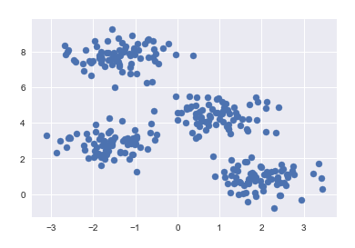
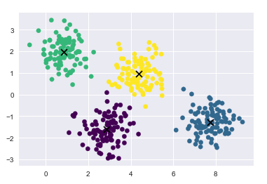
構造數據集

from sklearn.datasets.samples_generator import make_blobs
X, y_true = make_blobs(n_samples=300, centers=4, cluster_std=0.60, random_state=0)
plt.scatter(X[:,0], X[:, 1], s=50)

技術分享圖片

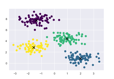
from sklearn.cluster import KMeans
kmeans = KMeans(n_clusters=4)
kmeans.fit(X)
y_kmeans = kmeans.predict(X)

繪制聚類結果，畫出聚類中心

plt.scatter(X[:, 0], X[:, 1], c=y_kmeans, s=50, cmap=‘viridis‘)

centers = kmeans.cluster_centers_
plt.scatter(centers[:,0], centers[:, 1], c=‘black‘, s=80, marker=‘x‘)

技術分享圖片

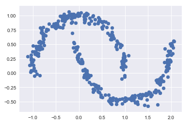
10.2 非線性邊界聚類

對於非線性邊界的kmeans聚類的介紹，查閱於《python數據科學手冊》P410

構造數據

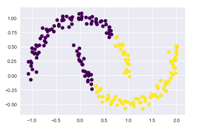
from sklearn.datasets import make_moons
X, y = make_moons(200, noise=0.05, random_state=0)

傳統kmeans聚類失敗的情況

labels = KMeans(n_clusters=2, random_state=0).fit_predict(X)
plt.scatter(X[:, 0], X[:, 1], c=labels, s=50, cmap=‘viridis‘)

技術分享圖片

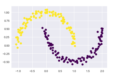
應用核方法，將數據投影到更高緯的空間，變成線性可分

from sklearn.cluster import SpectralClustering
model = SpectralClustering(n_clusters=2, affinity=‘nearest_neighbors‘, assign_labels=‘kmeans‘)
labels = model.fit_predict(X)
plt.scatter(X[:, 0], X[:, 1], c=labels, s=50, cmap=‘viridis‘)

技術分享圖片

10.3 預測結果與真實標簽的匹配

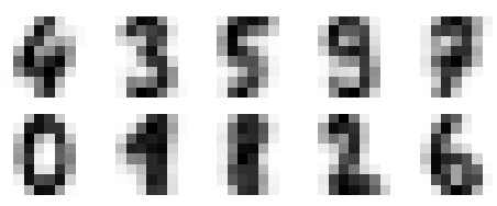
手寫數字識別例子

from sklearn.datasets import load_digits
digits = load_digits()

進行聚類

kmeans = KMeans(n_clusters=10, random_state=0)
clusters = kmeans.fit_predict(digits.data)
kmeans.cluster_centers_.shape
(10, 64)

可以將這些族中心點看做是具有代表性的數字

fig, ax = plt.subplots(2, 5, figsize=(8, 3))
centers = kmeans.cluster_centers_.reshape(10, 8, 8)
for axi, center in zip(ax.flat, centers):
    axi.set(xticks=[], yticks=[])
    axi.imshow(center, interpolation=‘nearest‘, cmap=plt.cm.binary)

技術分享圖片

進行眾數匹配

from scipy.stats import mode

labels = np.zeros_like(clusters)
for i in range(10):
    #得到聚類結果第i類的 True Flase 類型的index矩陣
    mask = (clusters ==i)
    #根據index矩陣，找出這些target中的眾數，作為真實的label
    labels[mask] = mode(digits.target[mask])[0]
#有了真實的指標，可以進行准確度計算

accuracy_score(digits.target, labels)
0.7935447968836951

10.4 聚類結果的混淆矩陣

from sklearn.metrics import confusion_matrix
mat = confusion_matrix(digits.target, labels)
np.fill_diagonal(mat, 0)
sns.heatmap(mat.T, square=True, annot=True, fmt=‘d‘, cbar=False,
            xticklabels=digits.target_names,
            yticklabels=digits.target_names)
plt.xlabel(‘true label‘)
plt.ylabel(‘predicted label‘)

技術分享圖片

10.5 t分布鄰域嵌入預處理

即將高緯的非線性的數據

通過流形學習

投影到低維空間

from sklearn.manifold import TSNE

# 投影數據
# 此過程比較耗時
tsen = TSNE(n_components=2, init=‘pca‘, random_state=0)
digits_proj = tsen.fit_transform(digits.data)

#計算聚類的結果
kmeans = KMeans(n_clusters=10, random_state=0)
clusters = kmeans.fit_predict(digits_proj)

#將聚類結果和真實標簽進行匹配
labels = np.zeros_like(clusters)
for i in range(10):
    mask = (clusters == i)
    labels[mask] = mode(digits.target[mask])[0]
    
# 計算准確度
accuracy_score(digits.target, labels)

11. 高斯混合模型（聚類、密度估計）

k-means算法的非概率性和僅根據到族中心的距離指派族的特征導致該算法性能低下

且k-means算法只對簡單的，分離性能好的，並且是圓形分布的數據有比較好的效果

本例中所有代碼的實現已上傳至 git倉庫

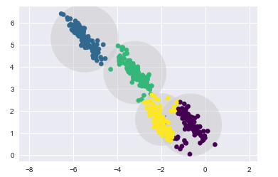
11.1 觀察K-means算法的缺陷

通過實例來觀察K-means算法的缺陷

%matplotlib inline
import matplotlib.pyplot as plt
import seaborn as sns; sns.set()
import numpy as np
# 生成數據點
from sklearn.datasets.samples_generator import make_blobs
X, y_true = make_blobs(n_samples=400, centers=4,
                       cluster_std=0.60, random_state=0)
X = X[:, ::-1] # flip axes for better plotting
# 繪制出kmeans聚類后的標簽的結果
from sklearn.cluster import KMeans
kmeans = KMeans(4, random_state=0)
labels = kmeans.fit(X).predict(X)
plt.scatter(X[:, 0], X[:, 1], c=labels, s=40, cmap=‘viridis‘);

centers = kmeans.cluster_centers_
plt.scatter(centers[:,0], centers[:, 1], c=‘black‘, s=80, marker=‘x‘)

技術分享圖片

k-means算法相當於在每個族的中心放置了一個圓圈，（針對此處的二維數據來說）

半徑是根據最遠的點與族中心點的距離算出

下面用一個函數將這個聚類圓圈可視化

from sklearn.cluster import KMeans
from scipy.spatial.distance import cdist

def plot_kmeans(kmeans, X, n_clusters=4, rseed=0, ax=None):
    labels = kmeans.fit_predict(X)

    # plot the input data
    ax = ax or plt.gca()
    ax.axis(‘equal‘)
    ax.scatter(X[:, 0], X[:, 1], c=labels, s=40, cmap=‘viridis‘, zorder=2)


    # plot the representation of the KMeans model

    centers = kmeans.cluster_centers_
    ax.scatter(centers[:,0], centers[:, 1], c=‘black‘, s=150, marker=‘x‘)
    
    radii = [cdist(X[labels == i], [center]).max() for i, center in enumerate(centers)]
    #用列表推導式求出每一個聚類中心 i = 0, 1, 2, 3在自己的所屬族的距離的最大值
    #labels == i 返回一個布爾型index，所以X[labels == i]只取出i這個族類的數據點
    #求出這些數據點到聚類中心的距離cdist(X[labels == i], [center])  再求最大值 .max()
    
    
    for c, r in zip(centers, radii):
        ax.add_patch(plt.Circle(c, r, fc=‘#CCCCCC‘, lw=3, alpha=0.5, zorder=1))
#如果數據點不是圓形分布的

k-means算法的聚類效果就會變差

rng = np.random.RandomState(13)
# 這里乘以一個2,2的矩陣，相當於在空間上執行旋轉拉伸操作
X_stretched = np.dot(X, rng.randn(2, 2))

kmeans = KMeans(n_clusters=4, random_state=0)
plot_kmeans(kmeans, X_stretched)

技術分享圖片

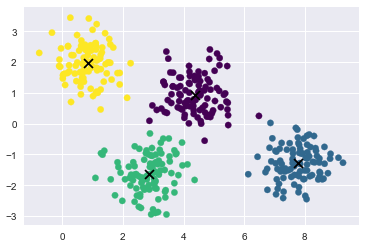
11.2 引出高斯混合模型

高斯混合模型能夠計算出每個數據點，屬於每個族中心的概率大小

在默認參數設置的、數據簡單可分的情況下，

GMM的分類效果與k-means基本相同

from sklearn.mixture import GaussianMixture
gmm = GaussianMixture(n_components=4).fit(X)
labels = gmm.predict(X)
plt.scatter(X[:, 0], X[:, 1], c=labels, s=40, cmap=‘viridis‘);


#gmm的中心點叫做 means_
centers = gmm.means_
plt.scatter(centers[:,0], centers[:, 1], c=‘black‘, s=80, marker=‘x‘);

得到數據的概率分布結果

probs = gmm.predict_proba(X)
print(probs[:5].round(3))
[[0.    0.469 0.    0.531]
 [1.    0.    0.    0.   ]
 [1.    0.    0.    0.   ]
 [0.    0.    0.    1.   ]
 [1.    0.    0.    0.   ]]

編寫繪制gmm繪制邊界的函數

from matplotlib.patches import Ellipse

def draw_ellipse(position, covariance, ax=None, **kwargs):
    """Draw an ellipse with a given position and covariance"""
    ax = ax or plt.gca()
    
    # Convert covariance to principal axes
    if covariance.shape == (2, 2):
        U, s, Vt = np.linalg.svd(covariance)
        angle = np.degrees(np.arctan2(U[1, 0], U[0, 0]))
        width, height = 2 * np.sqrt(s)
    else:
        angle = 0
        width, height = 2 * np.sqrt(covariance)
    
    # Draw the Ellipse
    for nsig in range(1, 4):
        ax.add_patch(Ellipse(position, nsig * width, nsig * height,
                             angle, **kwargs))
        
def plot_gmm(gmm, X, label=True, ax=None):
    ax = ax or plt.gca()
    labels = gmm.fit(X).predict(X)
    if label:
        ax.scatter(X[:, 0], X[:, 1], c=labels, s=40, cmap=‘viridis‘, zorder=2)
    else:
        ax.scatter(X[:, 0], X[:, 1], s=40, zorder=2)
    ax.axis(‘equal‘)
    
    w_factor = 0.2 / gmm.weights_.max()
    for pos, covar, w in zip(gmm.means_, gmm.covariances_, gmm.weights_):
        draw_ellipse(pos, covar, alpha=w * w_factor)

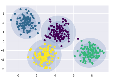
在圓形數據上的聚類結果

gmm = GaussianMixture(n_components=4, random_state=42)
plot_gmm(gmm, X)

技術分享圖片

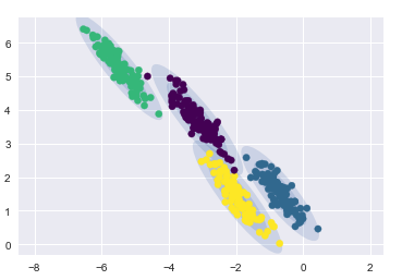
在偏斜拉伸數據上的聚類結果

gmm = GaussianMixture(n_components=4, covariance_type=‘full‘, random_state=42)
plot_gmm(gmm, X_stretched)

技術分享圖片

11.3 將GMM用作密度估計

GMM本質上是一個密度估計算法；也就是說，從技術的角度考慮，

一個 GMM 擬合的結果並不是一個聚類模型，而是描述數據分布的生成概率模型。

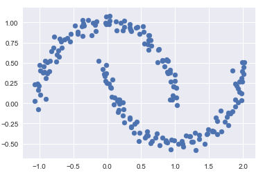
非線性邊界的情況

# 構建非線性可分數據

from sklearn.datasets import make_moons
Xmoon, ymoon = make_moons(200, noise=.05, random_state=0)
plt.scatter(Xmoon[:, 0], Xmoon[:, 1]);

技術分享圖片

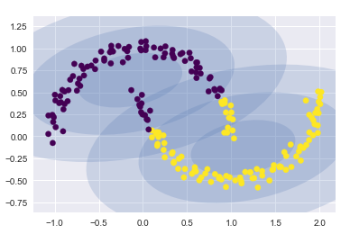
? 如果使用2個成分聚類（即廢了結果設置為2），基本沒什么效果

gmm2 = GaussianMixture(n_components=2, covariance_type=‘full‘, random_state=0)
plot_gmm(gmm2, Xmoon)

技術分享圖片

? 如果設置為多個聚類成分

gmm16 = GaussianMixture(n_components=16, covariance_type=‘full‘, random_state=0)
plot_gmm(gmm16, Xmoon, label=False)

技術分享圖片

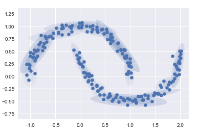
這里采用 16 個高斯曲線的混合形式不是為了找到數據的分隔的簇，而是為了對輸入數據的總體分布建模。

11.4 由分布函數得到生成模型

分布函數的生成模型可以生成新的，與輸入數據類似的隨機分布函數（生成新的數據點）

用 GMM 擬合原始數據獲得的 16 個成分生成的 400 個新數據點

Xnew = gmm16.sample(400)
Xnew[0][:5]
Xnew = gmm16.sample(400)
plt.scatter(Xnew[0][:, 0], Xnew[0][:, 1]);

技術分享圖片

11.5 需要多少成分？

作為一種生成模型，GMM 提供了一種確定數據集最優成分數量的方法。

赤池信息量准則（Akaike information criterion) AIC
貝葉斯信息准則（Bayesian information criterion) BIC

n_components = np.arange(1, 21)
models = [GaussianMixture(n, covariance_type=‘full‘, random_state=0).fit(Xmoon)
          for n in n_components]

plt.plot(n_components, [m.bic(Xmoon) for m in models], label=‘BIC‘)
plt.plot(n_components, [m.aic(Xmoon) for m in models], label=‘AIC‘)
plt.legend(loc=‘best‘)
plt.xlabel(‘n_components‘);

觀察可得，在 8~12 個主成分的時候，AIC 較小

評價指標

一、分類算法

常用指標選擇方式

平衡分類問題：

分類准確度、ROC曲線

類別不平衡問題：

精准率、召回率

對於二分類問題，常用的指標是 f1 、 roc_auc

多分類問題，可用的指標為 f1_weighted

1.分類准確度

一般用於平衡分類問題（每個類比的可能性相同）

from sklearn.metrics import accuracy_score
accuracy_score(y_test, y_predict)  #(真值，預測值)

2. 混淆矩陣、精准率、召回率

精准率：正確預測為1 的數量，占，所有預測為1的比例
召回率：正確預測為1 的數量，占， 所有確實為1的比例

# 先真實值，后預測值
from sklearn.metrics import confusion_matrix
confusion_matrix(y_test, y_log_predict)

from sklearn.metrics import precision_score
precision_score(y_test, y_log_predict)

from sklearn.metrics import recall_score
recall_score(y_test, y_log_predict)

多分類問題中的混淆矩陣

多分類結果的精准率

from sklearn.metrics import precision_score
precision_score(y_test, y_predict, average="micro")

多分類問題中的混淆矩陣

from sklearn.metrics import confusion_matrix

confusion_matrix(y_test, y_predict)

移除對角線上分類正確的結果，可視化查看其它分類錯誤的情況

同樣，橫坐標為預測值，縱坐標為真實值

cfm = confusion_matrix(y_test, y_predict)
row_sums = np.sum(cfm, axis=1)
err_matrix = cfm / row_sums
np.fill_diagonal(err_matrix, 0)

plt.matshow(err_matrix, cmap=plt.cm.gray)
plt.show()

3.F1-score

F1-score是精准率precision和召回率recall的調和平均數

from sklearn.metrics import f1_score

f1_score(y_test, y_predict)

4.精准率和召回率的平衡

可以通過調整閾值，改變精確率和召回率（默認閾值為0）

拉高閾值，會提高精准率，降低召回率
降低閾值，會降低精准率，提高召回率

# 返回模型算法預測得到的成績
# 這里是以  邏輯回歸算法  為例
decision_score = log_reg.decision_function(X_test)

# 調整閾值為5
y_predict_2 = np.array(decision_score >= 5, dtype=‘int‘)
# 返回的結果是0 、1

5.精准率-召回率曲線（PR曲線）

from sklearn.metrics import precision_recall_curve

precisions, recalls, thresholds = precision_recall_curve(y_test, decision_score)
# 這里的decision_score是上面由模型對X_test預測得到的對象

繪制PR曲線

# 精確率召回率曲線
plt.plot(precisions, recalls)
plt.show()

將精准率和召回率曲線，繪制在同一張圖中

注意，當取“最大的” threshold值的時候，精准率=1，召回率=0，

但是，這個最大的threshold沒有對應的值

因此thresholds會少一個

plt.plot(thresholds, precisions[:-1], color=‘r‘)
plt.plot(thresholds, recalls[:-1], color=‘b‘)
plt.show()

6.ROC曲線

Reciver Operation Characteristic Curve

TPR： True Positive rate
FPR： False Positive Rate

\[FPR=\frac{FP}{TN+FP} \]

繪制ROC曲線

from sklearn.metrics import roc_curve

fprs, tprs, thresholds = roc_curve(y_test, decision_scores)

plt.plot(fprs, tprs)
plt.show()

計算ROC曲線下方的面積的函數

roc_ area_ under_ curve_score

from sklearn.metrics import roc_auc_score

roc_auc_score(y_test, decision_scores)

曲線下方的面積可用於比較兩個模型的好壞

總之，上面提到的decision_score 是一個概率值，如0 1 二分類問題，應該是將每個樣本預測為1的概率，

如某個樣本的y_test為1，y_predict_probablity為0.875

每個測試樣本對應一個預測的概率值

通常在模型fit完成之后，都會有相應的得到概率的函數，如

model.predict_prob(X_test)

model.decision_function(X_test)

二、回歸算法

1.均方誤差 MSE

from sklearn.metrics import mean_squared_error
mean_squared_error(y_test, y_predict)

2.平均絕對值誤差 MAE

from sklearn.metrics import mean_absolute_error
mean_absolute_error(y_test, y_predict)

3.均方根誤差 RMSE

scikit中沒有單獨定於均方根誤差，需要自己對均方誤差MSE開平方根

4.R2評分

from sklearn.metrics import r2_score
r2_score(y_test, y_predict)

5.學習曲線

觀察模型在訓練數據集和測試數據集上的評分，隨着訓練數據集樣本數增加的變化趨勢。

import numpy as np
import matplot.pyplot as plt
from sklearn.metrics import mean_squared_error


def plot_learning_curve(algo, X_train, X_test, y_train, y_test):
    
    train_score = []
    test_score = []
    for i in range(1, len(X_train)+1):
        algo.fit(X_train[:i], y_train[:i])

        y_train_predict = algo.predict(X_train[:i])
        train_score.append(mean_squared_error(y_train[:i], y_train_predict))

        y_test_predict = algo.predict(X_test)
        test_score.append(mean_squared_error(y_test, y_test_predict))
    
    plt.plot([i for i in range(1, len(X_train)+1)], np.sqrt(train_score), label="train")
    plt.plot([i for i in range(1, len(X_train)+1)], np.sqrt(test_score), label="test")
    plt.legend()
    plt.axis([0,len(X_train)+1, 0, 4])

    plt.show()
 
# 調用
plot_learning_curve(LinearRegression(), X_train, X_test, y_train, y_test )

機器學習經典算法大全-代碼整理（python

免責聲明！

本站轉載的文章為個人學習借鑒使用，本站對版權不負任何法律責任。如果侵犯了您的隱私權益，請聯系本站郵箱yoyou2525@163.com刪除。

猜您在找 機器學習經典算法大全-代碼整理（python） Python3入門機器學習經典算法與應用資源機器學習10種經典算法的Python實現詳解十大經典機器學習算法——EM算法上手機器學習，從搞懂這十大經典算法開始機器學習與數據挖掘中的十大經典算法機器學習經典算法之KNN 機器學習的經典算法與應用機器學習經典算法之EM 機器學習經典算法之PageRank