用於超參數隨機化搜索的幾個分布

機器學習中超參數搜索的常用方法為 Grid Search，然而如果參數一多則容易碰到維數詛咒的問題，即參數之間的組合呈指數增長。如果有 \(m\) 個參數，每個有 \(n\) 個取值，則時間復雜度為 \(\Theta(n^m)\)。 Bengio 等人在 《Random Search for Hyper-Parameter Optimization》 中提出了隨機化搜索的方法。他們指出大部分參數空間存在 “低有效維度 (low effective dimensionality)” 的特點，即有些參數對目標函數影響較大，另一些則幾乎沒有影響。而且在不同的數據集中通常有效參數也不一樣。 在這種情況下 Random Search 通常效果較好，下圖是一個例子，其中只有兩個參數，綠色的參數影響較大，而黃色的參數則影響很小：

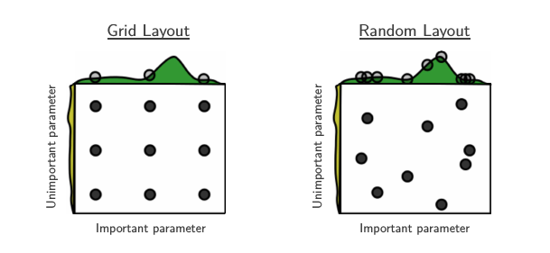
Grid Search 會評估每個可能的參數組合，所以對於影響較大的綠色參數，Grid Search 只探索了3個值，同時浪費了很多計算在影響小的黃色參數上； 相比之下 Random Search 則探索了9個不同的綠色參數值，因而效率更高，在相同的時間范圍內 Random Search 通常能找到更好的超參數 (當然這並不絕對)。 另外，Random Search 可以在連續的空間搜索，而 Grid Search 則只能在離散空間搜索，而對於像神經網絡中的 learning rate，SVM 中的 gamma 這樣的連續型參數宜使用連續分布。

在實際的應用中，Grid Search 只需為每個參數事先指定一個參數列表就可以了，而 Random Search 則通常需要為每個參數制定一個概率分布，進而從這些分布中進行抽樣。然而對什么樣的參數應該選擇什么樣的分布？這就大有講究了，如果選的分布不恰當可能就永遠找不到合適的參數值了，本文主要介紹一些超參數搜索的常用分布以及它們的特點和使用范圍。這些分布都出自 scipy.stats 模塊，共同特點是提供了 rvs 方法用於獨立隨機抽樣。

Randint 分布

Randint 分布的概率質量函數 (PMF) 為：

\[f(x) = \frac{1}{high - low} \]

其中 \(x = low,\,...,high - 1\) ，下面畫出隨機抽樣10000次后各個取值的分布圖：

np.random.seed(42)
randint = sp.stats.randint(low=-10, high=11)
randint_distribution = randint.rvs(size=10000, random_state=42)

start = randint.ppf(0.01)
end = randint.ppf(0.99)
x = np.arange(start, end+1)

randint_dict = dict(zip(*np.unique(randint_distribution, return_counts=True)))   # 計算各個數的頻次
randint_count = list(map(lambda x: x[1], sorted(list(randint_dict.items()), key=lambda x: x[0])))

plt.figure(figsize=(8,5))
plt.bar(x, randint_count, color='b', alpha=0.5, edgecolor='k',  label="random_samples")
plt.axhline(y=450, xmin=0.01, xmax=0.99, color='#FF00FF', linestyle="--")
plt.legend(frameon=False, fontsize=10)
plt.title("randint distribution", fontsize=17)
plt.show()

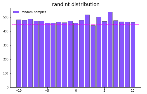
從上圖可以看出 Randint 分布為離散型均勻分布，適用於必須為整數的參數 (比如神經網絡的層數，決策樹的深度)。

Uniform 分布

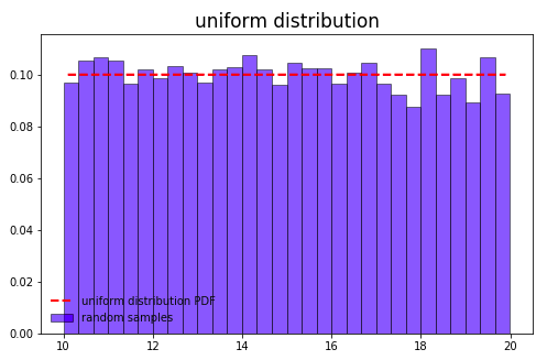
Uniform 是 Randint 分布的連續版本，概率密度函數為：

\[f(x) = \frac{1}{high - low} \]

其中 \(x \in [low, high]\)

np.random.seed(42)
uniform = sp.stats.uniform(loc=10, scale=10)
uniform_distribution = uniform.rvs(size=10000, random_state=42)
start = uniform.ppf(0.01)
end = uniform.ppf(0.99)
x = np.linspace(start, end, num=10000)

plt.figure(figsize=(8,5))
plt.plot(x, uniform.pdf(x), 'r--', lw=2, label="uniform distribution PDF")
plt.hist(uniform_distribution, bins=30, color='b', alpha=0.5, edgecolor = 'k', normed=True, label="random samples")
plt.legend(frameon=False, fontsize=10)
plt.title("uniform distribution", fontsize=17)
plt.show()

Geometric 分布

Geometric 分布的概率質量函數為 :

\[f(x) = (1-p)^{x-1} p \]

其中 \(x \geqslant 1\)

np.random.seed(42)
plt.figure(figsize=(8,5))
geom_distribution = sp.stats.geom.rvs(0.5, size=10000, random_state=42)
plt.hist(geom_distribution, bins=30, color='b', alpha=0.5, edgecolor = 'k', label="random samples")
plt.legend(frameon=False, fontsize=10)
plt.title("Geometric Distribution, p = 0.5", fontsize=17)
plt.show()

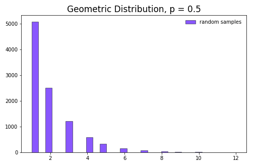
Geometric 分布為離散型分布，表示得到一次成功所需要的試驗次數，如果參數集中於少數幾個值且可能性呈離散型單調遞減，則適用此分布。

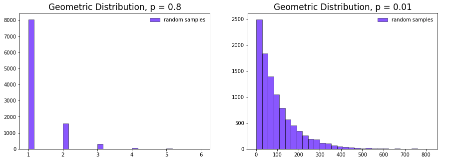
Geometric 分布概率質量函數中的 \(p\) 指定了一次試驗成功的概率。如果改變此值則會增大或縮小采樣范圍。

np.random.seed(42)
plt.figure(figsize=(15,5))
plt.subplot(121)
geom_distribution = sp.stats.geom.rvs(0.8, size=10000, random_state=42)
plt.hist(geom_distribution, bins=30, color='b', alpha=0.5, edgecolor = 'k', label="random samples")
plt.legend(frameon=False, fontsize=10)
plt.title("Geometric Distribution, p = 0.8", fontsize=17)

plt.subplot(122)
geom_distribution = sp.stats.geom.rvs(0.01, size=10000, random_state=42)
plt.hist(geom_distribution, bins=30, color='b', alpha=0.5, edgecolor = 'k', label="random samples")
plt.legend(frameon=False, fontsize=10)
plt.title("Geometric Distribution, p = 0.01", fontsize=17)
plt.show()

Exponential 分布

Exponential 分布是 Geometric 分布的連續版本，其概率密度函數為 ：

\[f(x) = e^{-x} \]

可以看到上圖中當Geometric 分布中的 \(p\) 非常小時，就會變得非常接近 exponential 分布。

plt.figure(figsize=(16,4))
expon_distribution = sp.stats.expon.rvs(loc=0, scale=1, size=10000, random_state=42)

plt.subplot(121)
start = sp.stats.expon.ppf(0.001)
end = sp.stats.expon.ppf(0.999)
x = np.linspace(start, end, num=10000)
plt.plot(x, sp.stats.expon.pdf(x), 'r--', lw=2, label=" exponential \ndistribution PDF")
plt.hist(expon_distribution, bins=30, color='b', alpha=0.5, edgecolor = 'k', normed=True, label="random samples")
plt.legend(frameon=False, fontsize=13)
plt.title("exponential distribution", fontsize=17)

plt.subplot(122)
plt.hist(np.log(expon_distribution), bins=30, edgecolor = 'k', color='b', alpha=0.5)
plt.title("log of exponential distribution", fontsize=17)
plt.axvline(x=-5, color='#FF00FF', linestyle="--")
plt.axvline(x=2, color='#FF00FF', linestyle="--")
plt.show()

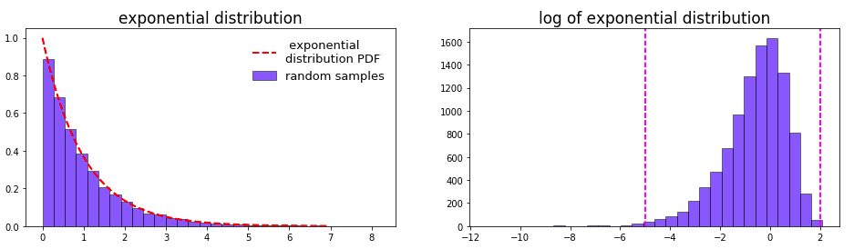
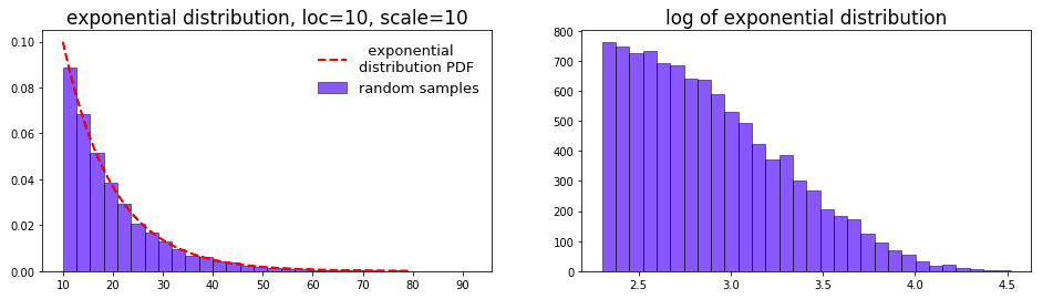
從右邊的 log 分布圖來看，大部分值集中於 \(e^{-5}\) 到 \(e^2\) 之間，即 \(0.0067 \sim 7.389\) 。如果有一些先驗知識，知道參數在0附近，且值越大可能性越小 (如svm中的gamma)，則適用此分布。當然也可以調整位置 (loc) 和 比例 (scale) 參數來改變搜索范圍。此時對應的概率密度函數為 (下面演示 loc=10，scale=10 的情況)：

\[f(x) = \frac{e^{-\frac{x - loc}{scale}}}{scale} \]

Reciprocal 分布

reciprocal 分布的概率密度函數為：

\[f(x, a, b) = \frac{1}{x \text{log}(b/a)} = \frac{1}{x\text{log}b - x\text{log}a} \]

其中 \(a < x < b, \; b > a > 0\)

np.random.seed(42)
plt.figure(figsize=(15,5))
reciprocal = sp.stats.reciprocal(a=0.1, b=100)
reciprocal_distribution = reciprocal.rvs(size=10000, random_state=42)

plt.subplot(121)
start = reciprocal.ppf(0.3)
end = reciprocal.ppf(0.99)
x = np.linspace(start, end, num=10000)
plt.plot(x, reciprocal.pdf(x), 'r--', lw=2, label="  reciprocal \ndistribution PDF")
plt.hist(reciprocal_distribution, bins=30, color='b', alpha=0.5, edgecolor = 'k', normed=True, label="random samples")
plt.legend(frameon=False, fontsize=13)
plt.title("reciprocal distribution", fontsize=17)

plt.subplot(122)
plt.hist(np.log10(reciprocal_distribution), bins=30, color='b', alpha=0.5, edgecolor = 'k')
plt.title("log of reciprocal distribution", fontsize=17)
plt.show()

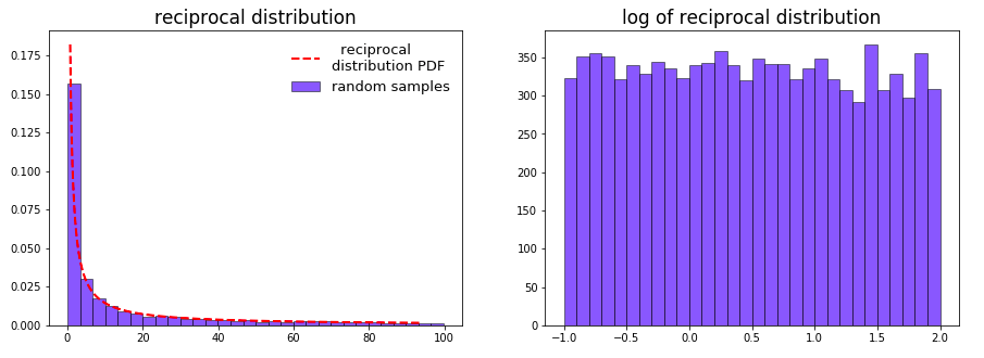
上圖中 reciprocal 分布的PDF和 exponential 分布比較相似，然而右邊的 log 分布圖卻是比較平均的，可見 reciprocal 分布是一個典型的對數均勻分布，以10為底為例，線性空間中10倍的差距在對數空間中均為1，設$x_2 = 10,x_1 $：

\[\begin{align*} \text{log}\,f(x_1, a, b) - \text{log}\, f(x_2, a, b) &= \text{log} \frac{1}{x_1 \text{log}(b/a)} - \text{log} \frac{1}{x_2 \text{log}(b/a)} \\[1ex] & = -\text{log} \, [x_1\text{log}(b/a)] + \text{log} \, [x_2\text{log}(b/a)] \\[1ex] & = -\text{log}\, x_1 + \text{log} \, x_2 \\[1ex] & = \text{log} \frac{x_2}{x_1} = 1 \end{align*} \]

下面用 np.random.uniform 可以模擬類似的分布。

np.random.seed(42)
log_uniform = 10 ** np.random.uniform(-1, 2, size=10000)

plt.figure(figsize=(15,5))
plt.subplot(121)
plt.hist(log_uniform, bins=30, color='b', alpha=0.5, normed=True, edgecolor='k')
plt.title("$10^{(-1 \sim 2)}$ distribution", fontsize=17)

plt.subplot(122)
plt.hist(np.log10(log_uniform), bins=30, color='b', alpha=0.5, edgecolor='k')
plt.title("log of $10^{(-1 \sim 2)}$ distribution", fontsize=17)
plt.show()

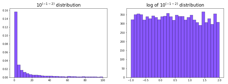
這種分布的好處是在不同的取值范圍內也能均勻地抽樣。如上圖中參數 \(x\) 的取值范圍是 \(0.1 \sim 100\)， 即 \(10^{-1} \sim 10^2\)，如果是一般的均勻分布中抽樣，\(10 \sim 100\) 這個范圍被取樣到的概率會遠大於 \(1 \sim 10\) 和 \(0.1 \sim 1\) 這兩個范圍，因為前者的距離更大，但在對數均勻分布中三者的范圍卻是一樣的，都是10的倍數，這樣被抽樣到的概率也就類似。下面的代碼顯示一個例子：

a = 0
b = 0
c = 0

reciprocal_distribution = sp.stats.reciprocal.rvs(a=0.1, b=100, size=10000, random_state=42)

for val in reciprocal_distribution:
    if val > 10 and val < 100:
        a += 1
    elif val > 1 and val < 10:
        b += 1
    elif val > 0.1 and val < 1:
        c +=1

print("10  到 100 之間取樣 {} 次".format(a))  # 10 到 100 之間取樣 3233 次
print("1   到 10  之間取樣 {} 次".format(b))  # 1 到 10 之間取樣 3392 次
print("0.1 到 1  之間取樣 {} 次".format(c))   # 0.1 到 1 之間取樣 3375 次

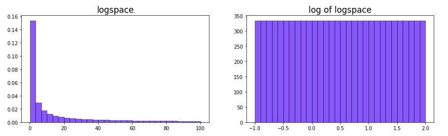
對於像 learning rate 這樣的參數，我們希望 \(0.01\sim0.1\) 和 \(0.1\sim1\) 范圍之間的抽樣概率是類似的。舉例來說，0.11和0.1的學習率可能相差不大，但0.01和0.02的學習率結果更可能大不相同，雖然這兩個范圍的絕對差異均為0.01。因此在這樣的參數中不同值之間的比率更適合作為超參數變化范圍。 另外實際上我們可以做到 “完全” 的對數均勻分布，這要用到 numpy 中的 logspace。 然而使用 np.logspace 的缺點是只能生成一個間隔均勻的固定數組進行采樣，從而喪失了一定的隨機性。

logspace = np.logspace(-1, 2, base=10, num=10000)
plt.figure(figsize=(15,4))
plt.subplot(121)
plt.hist(logspace, bins=30, color='b', alpha=0.5, normed=True, edgecolor='k')
plt.title("logspace", fontsize=17)
plt.subplot(122)
plt.hist(np.log10(logspace), bins=30, color='b', alpha=0.5, edgecolor='k')
plt.title("log of logspace", fontsize=17)
plt.show()

---

最后用scikit-learn中的 RandomizedSearchCV 來比較一下 Grid Search 和 Random Search 的效果，使用了 Kaggle 上的 HousePrices 比賽中的一個 Kernel 進行數據預處理，最后的特征數為410，使用的模型為超參數較多的 GBDT，評估指標為 RMSE：

1. 樹的數量 (n_estimators)
2. 損失函數類型 (loss)
3. 學習率 (learning_rate)
4. 子采樣率 (subsample)
5. 葉結點上的最少樣本數 (min_samples_leaf)
6. 最大深度 (max_depth)
7. 分裂時考慮的特征數 (max_features)

下面先嘗試 GridSearchCV

from sklearn.model_selection import GridSearchCV, RandomizedSearchCV

def neg_sqrt(val):  # 定義 RMSE
    return np.sqrt(-val)

model = GradientBoostingRegressor()
param_grid = {
    "learning_rate": [0.01, 0.05, 0.1],
    "n_estimators": [400, 800, 1500],
    "subsample": [0.8, 1.0],
    "max_depth": [2, 3, 4], 
    "max_features": [0.8, 1.0], 
    "min_samples_leaf": [1, 2],
    "loss": ["ls", "huber"],
    "random_state": [42],
}

grid_search = GridSearchCV(model, param_grid, scoring="neg_mean_squared_error", cv=5, verbose=3, n_jobs=-1)
grid_search.fit(X_scaled, y_log)
print("最優參數為: ", grid_search.best_params_, '\n')
print("RMSE 為: ", neg_sqrt(grid_search.best_score_))

結果如下：

最優參數為:  {'min_samples_leaf': 2, 'learning_rate': 0.05, 'max_depth': 2, 'random_state': 42, 'n_estimators': 1500, 'loss': 'huber', 'subsample': 0.8, 'max_features': 1.0} 

RMSE 為:  0.11852064590041982

上面過程中總共的參數組合為 \(3 \times 3 \times 2 \times 3 \times 2 \times 2 \times 2 = 432\) 個，接下來的RandomizedSearchCV 用了差不多的400個，其中 learning_rate 用了 reciprocal 這樣的對數均勻分布，原因前文已經說了。葉結點上的最少樣本數 (min_samples_leaf) 使用了 Geometric 分布，主要考慮到大部分值可能集中在 1和2左右。其他參數都使用均勻分布：

model = GradientBoostingRegressor()
param_distribution = {
    "learning_rate": sp.stats.reciprocal(a=0.01, b=0.1),  
    "n_estimators": sp.stats.randint(low=400, high=1500),
    "subsample": sp.stats.uniform(loc=0.8, scale=0.2),
    "max_depth": sp.stats.randint(low=2, high=4),
    "max_features": sp.stats.uniform(loc=0.8, scale=0.2),
    "min_samples_leaf": sp.stats.geom(p=0.6),
    "loss": ["ls", "huber"],
    "random_state": [42],
}

random_search = RandomizedSearchCV(model, param_distribution, n_iter=400, scoring="neg_mean_squared_error", cv=5, 
                                   verbose=3, random_state=42, n_jobs=-1) 
random_search.fit(X_scaled, y_log)
print("最優參數為: ", random_search.best_params_, '\n')
print("RMSE 為: ", neg_sqrt(random_search.best_score_))

結果如下：

最優參數為:  {'min_samples_leaf': 3, 'learning_rate': 0.03181845026156779, 'max_depth': 2, 'random_state': 42, 'n_estimators': 1476, 'loss': 'huber', 'subsample': 0.8978905520555127, 'max_features': 0.8557292928473224} 

RMSE 為:  0.11835604958840028

在這個數據集上 Random Search 的效果確實比 Grid Search 稍好，當然前提是為每個參數都選擇合適的分布。

/