[翻譯] 提升樹算法的介紹（Introduction to Boosted Trees）

## 1. 有監督學習的要素

XGBoost 適用於有監督學習問題。在此類問題中，我們使用多特征的訓練數據集 \(x_i\) 去預測一個目標變量 \(y_i\) 。在專門學習樹模型前，我們先回顧一下有監督學習的基本要素。

Elements of Supervised Learning

XGBoost is used for supervised learning problems, where we use the training data (with multiple features) \(x_i\) to predict a target variable \(y_i\). Before we learn about trees specifically, let us start by reviewing the basic elements in supervised learning.

## 1.1 模型和參數

有監督學習的模型通常指這樣的數學結構：預測值 \(y_i\) 是由給定輸入值 \(x_i\) 決定的。一個常見的例子是線性模型，其中預測值 \(\hat{y}_i=\sum_j \theta_jx_{ij}\) 是一個對輸入特征值的加權線性組合。這個預測值可以有不同的解釋，這取決於任務是回歸還是分類。例如，在邏輯回歸中，可通過預測值的邏輯變換獲得樣本被歸為正面類別的概率；當我們需要將輸出進行排序時，預測值也可作為一個排序得分值。

參數是我們需要從數據中學習得到的非確定部分。在線性回歸問題中，參數就是系數 \(\theta\)。我們通常用 \(\theta\) 代表參數（事實上模型中有許多參數，這里只是粗淺的定義一下）。

Model and Parameters

The model in supervised learning usually refers to the mathematical structure of by which the prediction \(y_i\) is made from the input \(x_i\). A common example is a linear model, where the prediction is given as \(\hat{y}_i=\sum_j \theta_jx_{ij}\), a linear combination of weighted input features. The prediction value can have different interpretations, depending on the task, i.e., regression or classification. For example, it can be logistic transformed to get the probability of positive class in logistic regression, and it can also be used as a ranking score when we want to rank the outputs.
The parameters are the undetermined part that we need to learn from data. In linear regression problems, the parameters are the coefficients θ. Usually we will use θ to denote the parameters (there are many parameters in a model, our definition here is sloppy).

## 1.2 目標函數：訓練損失+正則項

通過謹慎地選則 \(y_i\)，我們可以表達各種各樣的任務，比如回歸、分類、排序。訓練模型意味着要尋求最佳參數 \(\theta\) 使得能夠最好地擬合訓練數據 \(x_i\) 和標簽 \(y_i\)。為了訓練模型，我們需要定義目標函數來衡量這個模型擬合數據的效果有多好。

目標函數的一個顯著特征是，它由訓練損失和正則項兩個部分組成：

\[obj(\theta)=L(\theta)+\Omega(\theta) \]

式中 \(L\) 是訓練損失函數，\(\Omega\) 是正則項。訓練損失函數衡量的是模型在該訓練數據集上的預測能力。\(L\) 通常選擇均方誤差，公式如下：

\[L(\theta) = \sum_i (y_i - \hat y_i)^2 \]

另一個常用的損失函數是邏輯損失（logistic loss），被用於邏輯回歸問題：

\[L(\theta)=\sum_i[y_i\ln(1+e^{-\hat y_i})+(1-y_i)ln(1+e^{\hat y_i})] \]

人們通常會忘記加正則項。實際上，正則項能夠控制模型的復雜度，這有助於避免過擬合問題。這聽起來有點抽象。讓我們考慮下圖中的這個問題：對於左上角圖片中給出的輸入數據，要求直觀地給出一個階梯函數的擬合結果，三個圖中哪個方案的擬合效果最好？

正確答案已用紅色標出了。你是否能夠直觀地感覺出這是一個合理的擬合結果？一般性的原則就是，我們希望得到一個既簡單又具備預測能力的模型。在機器學習領域，這兩者之間的折衷也被稱為偏差-方差權衡（bias-variance tradeoff）。

Objective Function: Training Loss + Regularization

With judicious choices for yi, we may express a variety of tasks, such as regression, classification, and ranking. The task of training the model amounts to finding the best parameters θ that best fit the training data xi and labels yi. In order to train the model, we need to define the objective function to measure how well the model fit the training data.
A salient characteristic of objective functions is that they consist two parts: training loss and regularization term:

\[obj(\theta)=L(\theta)+\Omega(\theta)$$where Lis the training loss function, and Ω is the regularization term. The training loss measures how predictive our model is with respect to the training data. A common choice of L is the mean squared error, which is given by $$L(\theta) = \sum_i (y_i - \hat y_i)^2$$Another commonly used loss function is logistic loss, to be used for logistic regression: $$L(\theta)=\sum_i[y_i\ln(1+e^{-\hat y_i})+(1-y_i)ln(1+e^{\hat y_i})]$$The regularization term is what people usually forget to add. The regularization term controls the complexity of the model, which helps us to avoid overfitting. This sounds a bit abstract, so let us consider the following problem in the following picture. You are asked to fit visually a step function given the input data points on the upper left corner of the image. Which solution among the three do you think is the best fit? The correct answer is marked in red. Please consider if this visually seems a reasonable fit to you. The general principle is we want both a simple and predictive model. The tradeoff between the two is also referred as bias-variance tradeoff in machine learning. <br/> ## 1.3 為什么介紹一般原則 上面介紹的內容是有監督學習的基本要素，它們自然而然地成為了機器學習工具包的基本組成部分。例如，你應該能夠描述梯度提升樹和隨機森林的相同點和不同點。以形式化方法理解這一過程，有助於我們理解正在學習的對象以及啟發式算法背后的原因，例如剪枝和平滑。 >**Why introduce the general principle?** > The elements introduced above form the basic elements of supervised learning, and they are natural building blocks of machine learning toolkits. For example, you should be able to describe the differences and commonalities between gradient boosted trees and random forests. Understanding the process in a formalized way also helps us to understand the objective that we are learning and the reason behind the heuristics such as pruning and smoothing. <br/> ## 2 決策樹集成 <br/> 介紹完有監督學習的要素，現在開始進入真正的樹模型。首先，了解一下XGBoost所選擇的模型是：**決策樹集成**（decision tree ensemble）。樹集成模型包含了一組分類和回歸樹（CART）。下圖展示了一個CART用於對“某人是否會喜歡電腦游戲”分類的簡單例子。 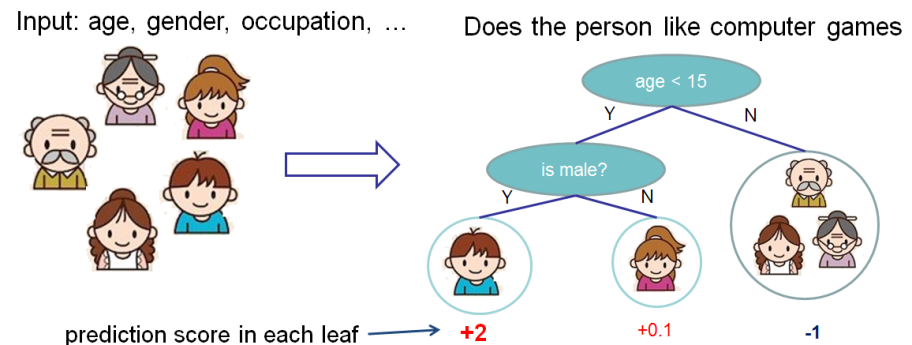 我們將一個家庭的成員划分入不同的葉子節點，並且給他們分配所在葉子節點相對應的分數。與葉子節點僅包含了決策值的決策樹不同，在CART中，一個實數分值是與每個葉節點相關聯的，這點比起分類器能讓我們對結果有更深的理解。正如我們將在接下來的章節會看到的那樣，這也使得能夠從原理上、以更統一的方式去做優化。 通常而言，單棵樹的能力是不夠直接被應用在實踐中的，實踐中運用的是集成模型，即將多棵樹的預測值求和。 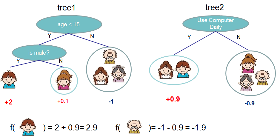 這是一個由兩棵樹構成的樹集成示例，最終得分由單棵樹的預測分值求和得到。一個關鍵點是，這兩個樹所做的是試圖互相**補充**。形式上我們可以用以下公式來表示模型： $$\hat y_i=\sum_{k=1}^Kf_k(x_i),\ f_k\in F\]

式中\(K\)是樹的總數，\(f\)是屬於函數空間\(F\)的函數，\(F\)是所有可能的CART的集合。待優化的目標函數如下：

\[obj(\theta)=\sum_i^nl(y_i,\hat y_i)+\sum_{k=1}^K\Omega(f_k) \]

現在有個巧妙的問題：隨機森林使用的是什么模型？是樹集成！所以隨機森林和提升樹其實是同樣的模型，不同之處在於我們如何訓練它們。這就意味着，如果你想用樹集成來寫一個預測服務，只需要寫一個就好了，它既能用隨機森林又能用梯度提升樹（參見[Treelite][1]的實例），一個說明為什么有監督學習的元素會抖動的例子。

Decision Tree Ensembles

Now that we have introduced the elements of supervised learning, let us get started with real trees. To begin with, let us first learn about the model choice of XGBoost: decision tree ensembles. The tree ensemble model consists of a set of classification and regression trees (CART). Here’s a simple example of a CART that classifies whether someone will like computer games.
We classify the members of a family into different leaves, and assign them the score on the corresponding leaf. A CART is a bit different from decision trees, in which the leaf only contains decision values. In CART, a real score is associated with each of the leaves, which gives us richer interpretations that go beyond classification. This also allows for a pricipled, unified approach to optimization, as we will see in a later part of this tutorial.
Usually, a single tree is not strong enough to be used in practice. What is actually used is the ensemble model, which sums the prediction of multiple trees together.
Here is an example of a tree ensemble of two trees. The prediction scores of each individual tree are summed up to get the final score. If you look at the example, an important fact is that the two trees try to complement each other. Mathematically, we can write our model in the form

\[\hat y_i=\sum_{k=1}^Kf_k(x_i),\ f_k\in F$$where K is the number of trees, f is a function in the functional space F, and F is the set of all possible CARTs. The objective function to be optimized is given by $$obj(\theta)=\sum_i^nl(y_i,\hat y_i)+\sum_{k=1}^K\Omega(f_k)$$Now here comes a trick question: what is the model used in random forests? Tree ensembles! So random forests and boosted trees are really the same models; the difference arises from how we train them. This means that, if you write a predictive service for tree ensembles, you only need to write one and it should work for both random forests and gradient boosted trees. (See Treelite for an actual example.) One example of why elements of supervised learning rock. <br/> ## 3 樹提升 <br/> 已經介紹完了模型，接下來我們把目光聚焦在訓練上：我們要如何學習出這些樹呢？答案是，正如所有有監督學習模型一直做的事：**定義一個目標函數然后做優化**。 現在假設下面這個函數是我們的目標函數（記得它始終需要含有訓練損失和正則項）： $$obj=\sum_{i=1}^nl(y_i,\hat y_i^{(t)})+\sum_{k=1}^t\Omega(f_i)\]

Tree Boosting
Now that we introduced the model, let us turn to training: How should we learn the trees? The answer is, as is always for all supervised learning models: define an objective function and optimize it!
Let the following be the objective function (remember it always needs to contain training loss and regularization):

\[obj=\sum_{i=1}^nl(y_i,\hat y_i^{(t)})+\sum_{k=1}^t\Omega(f_i) \]

## 3.1 累加訓練

我們會想詢問的第一個問題是：樹的參數有哪些？你會發現我們需要學習得到的就是那些函數\(f_i\)，每個都包含了樹結構及葉節點分數。學習樹結構比傳統的最優化問題難多了，在傳統最優化問題中只需要簡單地取梯度就好。一次性地學習出所有的樹是很難解決的。作為替代，我們使用累加策略：保持已經得到的訓練結果不變，僅僅在每次訓練時增加一棵新的樹。設第\(t\)步中得到的預測值是\(\hat y_i^{(t)}\)。那么我們有：

\[\begin{split} \hat y_i^{(0)}&=0\\ \hat y_i^{(1)}&=f_1(x_i)=\hat y_i^{(0)}+f_1(x_i)\\ \hat y_i^{(2)}&=f_1(x_i)+f_2(x_i)=\hat y_i^{(1)}+f_2(x_i)\\ &...\\ \hat y_i^{(t)}&=\sum_{k=1}^tf_k(x_i)=\hat y_i^{(t-1)}+f_t(x_i) \end{split} \]

還有一個問題：在每步中加入的樹要怎么選？一個很自然的想法就是加入那棵能夠最優化我們的目標函數的樹。

\[\begin{split} obj^{(t)}&=\sum_{i=1}^nl(y_i,\hat y_i^{(t)})+\sum_{k=1}^t\Omega(f_i)\\ &=\sum_{i=1}^nl(y_i,\hat y_i^{(t-1)}+f_t(x_i))+\Omega(f_t)+constant \end{split} \]

如果考慮使用均方差（MSE）作為損失函數，那么目標就變為：

\[\begin{split} obj^{(t)}&=\sum_{i=1}^n(y_i-(\hat y_i^{(t-1)}+f_t(x_i)))^2+\sum_{i=1}^t\Omega(f_i)\\ &=\sum_{i=1}^n[2(\hat y_i^{(t-1)}-y_i)f_t(x_i)+f_t(x_i)^2]+\Omega(f_t)+constant \end{split} \]

MSE的公式非常友好，有一個一次性（通常稱為殘差）和一個二次項。如果使用其他損失函數（比如邏輯損失），就很難得到這么漂亮的公式了。因此在這個一般情況下，我們對損失函數進行二次泰勒展開：

\[obj^{(t)}=\sum_{i=1}^n[l(y_i,\hat y_i^{(t-1)})+g_if_t(x_i)+\frac{1}{2}h_if_t^2(x_i)]+\Omega(f_t)+constant \]

式中\(g_i\)和\(h_i\)的定義是：

\[g_i=\partial_{\hat y_i^{(t-1)}} l(y_i,\hat y_i^{(t-1)})\\ h_i=\partial_{\hat y_i^{(t-1)}}^2 l(y_i,\hat y_i^{(t-1)}) \]

移除所有常數項后，在第\(t\)步中的特定目標即為：

\[\sum_{i=1}^n[g_if_t(x_i)+\frac{1}{2}h_if_t^2(x_i)]+\Omega(f_t) \]

這就是我們構造新樹的最優化目標。這一定義帶來的一個重要優勢是，目標函數值僅取決於\(g_i\)和\(h_i\)，這就是XGBoost能夠支持自定義目標函數的原因。我們能夠優化所有損失函數，包括邏輯回歸和pairwise排序，對於不同的輸入值\(g_i\)和\(h_i\)使用的是完全一致的解決方案。

Additive Training

The first question we want to ask: what are the parameters of trees? You can find that what we need to learn are those functions \(f_i\), each containing the structure of the tree and the leaf scores. Learning tree structure is much harder than traditional optimization problem where you can simply take the gradient. It is intractable to learn all the trees at once. Instead, we use an additive strategy: fix what we have learned, and add one new tree at a time. We write the prediction value at step t as \(\hat y_i^{(t)}\). Then we have

\[\begin{split} \hat y_i^{(0)}&=0\\ \hat y_i^{(1)}&=f_1(x_i)=\hat y_i^{(0)}+f_1(x_i)\\ \hat y_i^{(2)}&=f_1(x_i)+f_2(x_i)=\hat y_i^{(1)}+f_2(x_i)\\ &...\\ \hat y_i^{(t)}&=\sum_{k=1}^tf_k(x_i)=\hat y_i^{(t-1)}+f_t(x_i) \end{split} $$It remains to ask: which tree do we want at each step? A natural thing is to add the one that optimizes our objective. \]

\begin{split}
obj^{(t)}&=\sum_{i=1}^nl(y_i,\hat y_i^{(t)})+\sum_{k=1}^t\Omega(f_i)\
&=\sum_{i=1}^nl(y_i,\hat y_i^{(t-1)}+f_t(x_i))+\Omega(f_t)+constant
\end{split}

\[If we consider using mean squared error (MSE) as our loss function, the objective becomes \]

\begin{split}
obj^{(t)}&=\sum_{i=1}^n(y_i-(\hat y_i^{(t-1)}+f_t(x_i)))^2+\sum_{i=1}^t\Omega(f_i)\
&=\sum_{i=1}^n[2(\hat y_i^{(t-1)}-y_i)f_t(x_i)+f_t(x_i)^2]+\Omega(f_t)+constant
\end{split}

\[The form of MSE is friendly, with a first order term (usually called the residual) and a quadratic term. For other losses of interest (for example, logistic loss), it is not so easy to get such a nice form. So in the general case, we take the Taylor expansion of the loss function up to the second order: $$obj^{(t)}=\sum_{i=1}^n[l(y_i,\hat y_i^{(t-1)})+g_if_t(x_i)+\frac{1}{2}h_if_t^2(x_i)]+\Omega(f_t)+constant$$where the $g_i$ and $h_i$ are defined as \]

g_i=\partial_{\hat y_i^{(t-1)}} l(y_i,\hat y_i^{(t-1)})\
h_i=\partial_{\hat y_i^{(t-1)}}^2 l(y_i,\hat y_i^{(t-1)})

\[After we remove all the constants, the specific objective at step t becomes $$\sum_{i=1}^n[g_if_t(x_i)+\frac{1}{2}h_if_t^2(x_i)]+\Omega(f_t)$$This becomes our optimization goal for the new tree. One important advantage of this definition is that the value of the objective function only depends on $g_i$ and $h_i$. This is how XGBoost supports custom loss functions. We can optimize every loss function, including logistic regression and pairwise ranking, using exactly the same solver that takes $g_i$ and $h_i$ as input! <br/> ## 3.2 模型復雜度 介紹完了訓練步驟，但是稍等，還有一件很重要的事情，那就是**正則項**！我們需要為樹定義復雜度$\Omega(f)$。為了做這件事，讓我們改進一下對於樹$f(x)$的定義： $$f_t(x)=\omega_{q(x)},\ \omega \in R^T,\ q:R^d \rightarrow \{1,2,...,T\}\]

這里 \(\omega\) 是葉節點分值向量，\(q\)是將每個數據點分配到相對應的葉節點中去的函數，\(T\)是葉子數量。在XGBoost中，我們定義復雜度如下：

\[\Omega (f)=\gamma T+\frac{1}{2}\lambda\sum_{j=1}^T\omega_j^2 \]

當然，還有其他多種方式來定義復雜度，但是上式的定義在實踐中效果最好。正則項是被大多數樹算法的包粗略對待甚至直接忽視的一部分內容。這是因為傳統對於樹的學習只重視改善不純度，而對復雜度的控制就留給了啟發式算法。通過形式化地定義正則項，我們能夠對正在學習的東西有更好的認識，並得到一個更加泛化的模型。

Model Complexity

We have introduced the training step, but wait, there is one important thing, the regularization term! We need to define the complexity of the tree Ω(f). In order to do so, let us first refine the definition of the tree f(x) as

\[f_t(x)=\omega_{q(x)},\ \omega \in R^T,\ q:R^d \rightarrow \{1,2,...,T\}$$Here w is the vector of scores on leaves, q is a function assigning each data point to the corresponding leaf, and T is the number of leaves. In XGBoost, we define the complexity as $$\Omega (f)=\gamma T+\frac{1}{2}\lambda\sum_{j=1}^T\omega_j^2$$Of course, there is more than one way to define the complexity, but this one works well in practice. The regularization is one part most tree packages treat less carefully, or simply ignore. This was because the traditional treatment of tree learning only emphasized improving impurity, while the complexity control was left to heuristics. By defining it formally, we can get a better idea of what we are learning and obtain models that perform well in the wild. <br/> ## 3.3 結構分數 導數中有一個神奇的部分。在重構樹模型后，我們可以將第$t$棵樹的目標值寫作： \]

\begin{split}
obj^{(t)}&\approx \sum_{i=1}^n[g_i\omega_{q(x_i)}+\frac{1}{2}h_i\omega_{q(x_i)}^2]+\gamma T+\frac{1}{2}\lambda\sum_{j=1}^T\omega_j^2\
&=\sum_{j=1}^T[(\sum_{i \in I_j}g_i)\omega_j+\frac{1}{2}(\sum_{i \in I_j}h_i+\lambda)\omega_j^2]+\gamma T
\end{split}

\[ 式中 $I_j=\{i \mid q(x_i)=j\}$ 是被分配到第$j$個葉子的數據點的下標集合。注意到在第二行中，我們變換了求和函數的下標，因為位於同個葉子中的所有數據點得到的分值是相同的。更近一步化簡表達式，定義$G_j=\sum_{i \in I_j}g_i$，$H_j=\sum_{i \in I_j}h_i$，得到： $$obj^{(t)}=\sum_{j=1}^T[G_j\omega_j+\frac{1}{2}(H_j+\lambda)\omega_j^2]+\gamma T\]

在這一等式中，\(w_j\)是互相獨立的，式子\(G_j\omega_j+\frac{1}{2}(H_j+\lambda)\omega_j^2\)是一個二次項。對於給定的結構\(q(x)\)，使目標函數的最小化的\(\omega_j\)的取值、及最小化的目標函數為：

\[\begin{split} \omega_j^*&=-\frac{G_j}{H_j+\lambda}\\ obj^*&=-\frac{1}{2}\sum_{j=1}^T\frac{G_j^2}{H_j+\lambda}+\gamma T \end{split} \]

后一個等式衡量了樹結構\(q(x)\)有多好。

如果所有這些聽起來有點復雜，讓我們看看在這張圖片中，分數是怎樣計算得出的。總的來說，對於一個給定的樹結構，我們將定值\(g_i\)和\(h_i\)放到它們對應的葉節點中，將這些值求和，然后運用公式計算出這棵樹有多好。這個得分很像決策樹中的不純度，只是它將模型復雜度也考慮進去了。

The Structure Score

Here is the magical part of the derivation. After re-formulating the tree model, we can write the objective value with the t-th tree as:

\[\begin{split} obj^{(t)}&\approx \sum_{i=1}^n[g_i\omega_{q(x_i)}+\frac{1}{2}h_i\omega_{q(x_i)}^2]+\gamma T+\frac{1}{2}\lambda\sum_{j=1}^T\omega_j^2\\ &=\sum_{j=1}^T[(\sum_{i \in I_j}g_i)\omega_j+\frac{1}{2}(\sum_{i \in I_j}h_i+\lambda)\omega_j^2]+\gamma T \end{split} $$where $I_j=\{i|q(xi)=j\}$ is the set of indices of data points assigned to the j-th leaf. Notice that in the second line we have changed the index of the summation because all the data points on the same leaf get the same score. We could further compress the expression by defining $G_j=\sum_{i \in I_j}g_i$ and $H_j=\sum_{i \in I_j}h_i$ : $$obj^{(t)}=\sum_{j=1}^T[G_j\omega_j+\frac{1}{2}(H_j+\lambda)\omega_j^2]+\gamma T$$In this equation, $w_j$ are independent with respect to each other, the form $G_j\omega_j+\frac{1}{2}(H_j+\lambda)\omega_j^2$ is quadratic and the best wj for a given structure q(x) and the best objective reduction we can get is: \]

\begin{split}
\omega_j^&=-\frac{G_j}{H_j+\lambda}\
obj^&=-\frac{1}{2}\sum_{j=1}^T\frac{G_j^2}{H_j+\lambda}+\gamma T
\end{split}

\[The last equation measures how good a tree structure q(x) is. If all this sounds a bit complicated, let’s take a look at the picture, and see how the scores can be calculated. Basically, for a given tree structure, we push the statistics gi and hi to the leaves they belong to, sum the statistics together, and use the formula to calculate how good the tree is. This score is like the impurity measure in a decision tree, except that it also takes the model complexity into account. <br/> ## 3.4 學習樹結構 既然我們已有了衡量一棵樹有多好的方法，理論上我們可以枚舉所有可能的樹然后挑出最好的，但在實際中這是很難做到的，所以我們將嘗試每次優化樹的一層。 特別地，若我們試圖將一個葉節點划分為兩個葉節點，此時分數增益為： $$Gain=\frac{1}{2}[\frac{G_L^2}{H_L+\lambda}+\frac{G_R^2}{H_R+\lambda}-\frac{(G_L+G_R)^2}{H_L+H_R+\lambda}]-\gamma\]

這個公式可被拆分為 1)左子樹得分 2）右子樹得分 3) 原葉節點得分 4）對新增添的葉子的正則化項。顯而易見的是，如果增益值比\(\gamma\)值小，我們就最好不要添加這個分支。這也正是所有基於樹的模型的剪枝技術。通過運用有監督學習的原則，我們自然能想到這些技術能夠起效果的原因 : )

對於實數值的數據，我們通常想要找到最優的切分點。為了高效地做這件事，我們先將所有樣本排序好，像下圖所示：

只要從左到右掃描，就足夠用於計算所有可能的切分方案的結構分數，然后我們就能高效地找到最佳切分點。

Learn the tree structure

Now that we have a way to measure how good a tree is, ideally we would enumerate all possible trees and pick the best one. In practice this is intractable, so we will try to optimize one level of the tree at a time. Specifically we try to split a leaf into two leaves, and the score it gains is

\[Gain=\frac{1}{2}[\frac{G_L^2}{H_L+\lambda}+\frac{G_R^2}{H_R+\lambda}-\frac{(G_L+G_R)^2}{H_L+H_R+\lambda}]-\gamma$$This formula can be decomposed as 1) the score on the new left leaf 2) the score on the new right leaf 3) The score on the original leaf 4) regularization on the additional leaf. We can see an important fact here: if the gain is smaller than γ , we would do better not to add that branch. This is exactly the pruning techniques in tree based models! By using the principles of supervised learning, we can naturally come up with the reason these techniques work :) For real valued data, we usually want to search for an optimal split. To efficiently do so, we place all the instances in sorted order, like the following picture. A left to right scan is sufficient to calculate the structure score of all possible split solutions, and we can find the best split efficiently. <br/> --- 關於公式推導中常數項的解釋：在第t步時，前t-1步的運算結果都可視作已知（常數）。 原文：[Introduction to Boosted Trees][2] 相關概念閱讀參考： [Understanding the Bias-Variance Tradeoff][3] [分類與回歸樹（Classification and Regression Trees, CART）][4] [L1, L2 Regularization – Why needed/What it does/How it helps?][5] 感謝南大薛愷豐同學幫忙校對~ [1]: https://treelite.readthedocs.io/en/latest/ [2]: https://xgboost.readthedocs.io/en/latest/tutorials/model.html [3]: https://towardsdatascience.com/understanding-the-bias-variance-tradeoff-165e6942b229 [4]: https://wizardforcel.gitbooks.io/dm-algo-top10/content/cart.html [5]: https://www.linkedin.com/pulse/l1-l2-regularization-why-neededwhat-doeshow-helps-ravi-shankar\]