TensorFlow: How to freeze a model and serve it with a python API
參考:https://blog.metaflow.fr/tensorflow-how-to-freeze-a-model-and-serve-it-with-a-python-api-d4f3596b3adc
官方的源碼:https://github.com/tensorflow/tensorflow/blob/master/tensorflow/python/tools/freeze_graph.py
We are going to explore two parts of using a ML model in production:
- How to export a model and have a simple self-sufficient file for it
- How to build a simple python server (using flask) to serve it with TF
Note: if you want to see the kind of graph I save/load/freeze, you can here
How to freeze (export) a saved model
If you wonder how to save a model with TensorFlow, please have a look at my previous article before going on.
let’s start from a folder containing a model, it probably looks something like this:
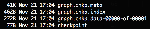
Screenshot of the result folder before freezing our model
The important files here are the “.chkp” ones. If you remember well, for each pair at different timesteps, one is holding the weights (“.data”) and the other one (“.meta”) is holding the graph and all its metadata (so you can retrain it etc…)
But when we want to serve a model in production, we don’t need any special metadata to clutter our files, we just want our model and its weights nicely packaged in one file. This facilitate storage, versioning and updates of your different models.
Luckily in TF, we can easily build our own function to do it. Let’s explore the different steps we have to perform:
- Retrieve our saved graph: we need to load the previously saved meta graph in the default graph and retrieve its graph_def (the ProtoBuf definition of our graph)
- Restore the weights: we start a Session and restore the weights of our graph inside that Session
- Remove all metadata useless for inference: Here, TF helps us with a nice helper function which grab just what is needed in your graph to perform inference and returns what we will call our new “frozen graph_def”
- Save it to the disk, Finally we will serialize our frozen graph_def ProtoBuf and dump it to the disk
Note that the two first steps are the same as when we load any graph in TF, the only tricky part is actually the graph “freezing” and TF has a built-in function to do it!
I provide a slightly different version which is simpler and that I found handy. The original freeze_graph function provided by TF is installed in your bin dir and can be called directly if you used PIP to install TF. If not you can call it directly from its folder (see the commented import in the gist).
So let’s see:
Now we can see a new file in our folder: “frozen_model.pb”.
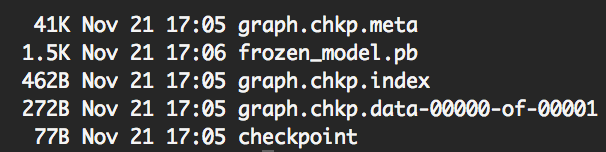
Screenshot of the result folder after freezing our model
As expected, its size is bigger than the weights file size and lower than the sum of the two checkpoints files sizes.
Note: In this very simple case, the weights size is very small, but it is usually multiple Mbs.
How to use the frozen model
Naturally, after knowing how to freeze a model, one might wonder how to use it.
The little trick to have in mind is to understand that what we dumped to the disk was a graph_def ProtoBuf. So to import it back in a python script we need to:
- Import a graph_def ProtoBuf first
- Load this graph_def into a actual Graph
We can build a convenient function to do so:
Now that we built our function to load our frozen model, let’s create a simple script to finally make use of it:
Note: when loading the frozen model, all operations got prefixed by “prefix”. This is due to the parameter “name” in the “import_graph_def” function, by default it prefix everything by “import”.
This can be useful to avoid name collisions if you want to import your graph_def in an existing Graph.
How to build a (very) simple API
For this part, I will let the code speaks for itself, after all this is a TF series about TF and not so much about how to build a server in python. Yet it felt kind of unfinished without it, so here you go, the final workflow:
Note: We are using flask in this example
TensorFlow best practice series
This article is part of a more complete series of articles about TensorFlow. I’ve not yet defined all the different subjects of this series, so if you want to see any area of TensorFlow explored, add a comment! So far I wanted to explore those subjects (this list is subject to change and is in no particular order):
- A primer
- How to handle shapes in TensorFlow
- TensorFlow saving/restoring and mixing multiple models
- How to freeze a model and serve it with python (this one!)
- TensorFlow: A proposal of good practices for files, folders and models architecture
- TensorFlow howto: a universal approximator inside a neural net
- How to optimise your input pipeline with queues and multi-threading
- Mutating variables and control flow
- How to handle input data with TensorFlow.
- How to control the gradients to create custom back-prop or fine-tune my models.
- How to monitor my training and inspect my models to gain insight about them.
Note: TF is evolving fast right now, those articles are currently written for the 1.0.0 version.
References
使用TensorFlow C++ API構建線上預測服務 - 第二篇
之前的一篇文章中使用TensorFlow C++ API構建線上預測服務 - 第一篇,詳細講解了怎樣用TensorFlow C++ API導入模型做預測,但模型c = a * b比較簡單,只有模型結構,並沒有參數,所以文章中並沒講到怎樣導入參數。本文使用一個復雜的模型講解,包括以下幾個方面:
- 針對稀疏數據的數據預處理
- 訓練中保存模型和參數
- TensorFlow C++ API導入模型和參數
- TensorFlow C++ API構造Sparse Tensor做模型輸入
稀疏數據下的數據預處理
稀疏數據下,一般會調用TensorFlow的embedding_lookup_sparse。
|
1
2
|
embedding_variable = tf.Variable(tf.truncated_normal([input_size, embedding_size], stddev=
0.05), name='emb')
embedding = tf.nn.embedding_lookup_sparse(embedding_variable, sparse_id, sparse_value,
"mod", combiner="sum")
|
上面代碼中,embedding_variable就是需要學習的參數,其中input_size是矩陣的行數,embedding_size是矩陣的列數,比如我們有100萬個稀疏id,每個id要embedding到50維向量,那么矩陣的大小是[1000000, 50]。sparse_id是要做向量化的一組id,用SparseTensor表示,sparse_value是每個id對用的一個value,用作權重,也用SparseTensor表示。
這里要注意,如果id是用hash生成的,不保證id是0,1,2,3, ...這種連續表示,需要先把id排序后轉成連續的,並且把input_size設成大於排序后最大的id,為了節省空間往往設成排序后最大id+1。因為用id去embedding_variable矩陣查詢命中哪行的時候,使用id mod Row(embedding_variable)或其他策略作為命中的行數,如果不保證id連續,可能會出現多個id命中同一行的錯誤情況。另外,如果不把id排序后轉成連續id,那input_size需要設成原始id中的最大id,如果是hash生成的那么最大id值非常大,做成矩陣非常大存不下和矩陣存在空間浪費,因為有些行肯定不會被命中。
另外一個點,目前TensorFlow不支持sparse方式的查詢和參數更新,每次查詢更新都要pull&push一個矩陣全量數據,造成網絡的堵塞,速度過慢,所以一般來說不要使用太大的embedding矩陣。
訓練中保存模型和參數
TensorFlow保存模型時分為兩部分,網絡結構和參數是分開保存的。
保存網絡結構
運行以下命令,成功后會看到一個名為graph.pb的pb二進制文件。后續如果使用TensorFlow官方提供的freeze_graph.py工具時必需這個文件,當然,如果對freeze_graph.py的代碼比較熟悉,可以使用比較trick的方式,這樣只需要參數文件,而不需要graph.pb了。
|
1
|
tf.train.write_graph(sess.graph.as_graph_def(), FLAGS.model_dir,
'graph.pb', as_text=False)
|
保存模型參數
運行以下命令,會在FLAGS.model_dir目錄下保存多個前綴為model.checkpoint的文件。
|
1
2
|
saver = tf.train.Saver()
saver.save(sess, FLAGS.model_dir +
"/model.checkpoint")
|
比如,成功后在FLAGS.model_dir目錄下會看到以下幾個文件。其中,model.checkpoint.meta包含了網絡結構和一些其他信息,所以也包含了上面提到的graph.pb;model.checkpoint.data-00000-of-00001保存了模型參數,其他兩個文件輔助作用。
|
1
2
3
4
|
-rw-r--r-- 1
user staff 89 10 11 11:32 checkpoint
-rw-r--r-- 1
user staff 225136 10 11 11:32 model.checkpoint.data-00000-of-00001
-rw-r--r-- 1
user staff 1506 10 11 11:32 model.checkpoint.index
-rw-r--r-- 1
user staff 369379 10 11 11:32 model.checkpoint.meta
|
TensorFlow C++ API導入模型和參數
主要有兩種方法:
- 分別導入網絡結構和模型參數
- 線下先把網絡結構和模型參數整合成一個文件,只用導入這個文件即可
分別導入網絡結構和模型參數
導入網絡結構
以上文的graph.pb為例
|
1
2
3
4
5
6
7
8
9
10
11
12
|
// 導入網絡結構
GraphDef graph_def;
status = ReadBinaryProto(Env::Default(),
std::string("graph.pb"), &graph_def);
if (!status.ok()) {
throw runtime_error("Error loading graph: " + status.ToString());
}
// 把網絡設置到Session里
status = session->Create(graph_def);
if (!status.ok()) {
throw runtime_error("Error set graph to session: " + status.ToString());
}
|
導入模型參數
這里注意要傳入模型路徑,既上文的FLAGS.model_dir。以FLAGS.model_dir="your_checkpoint_path"為例
|
1
2
3
4
5
6
7
8
9
10
11
|
// 導入模型參數
Tensor checkpointPathTensor(DT_STRING, TensorShape());
checkpointPathTensor.scalar<
std::string>()() = std::string("your_checkpoint_path");
status = session->Run(
{{ graph_def.saver_def().filename_tensor_name(), checkpointPathTensor },},
{},
{graph_def.saver_def().restore_op_name()},
nullptr);
if (!status.ok()) {
throw runtime_error("Error loading checkpoint: " + status.ToString());
}
|
網絡結構和模型參數整合成一個文件
One confusing part about this is that the weights usually aren’t stored inside the file format during training. Instead, they’re held in separate checkpoint files, and there are Variable ops in the graph that load the latest values when they’re initialized. It’s often not very convenient to have separate files when you’re deploying to production, so there’s the freeze_graph.py script that takes a graph definition and a set of checkpoints and freezes them together into a single file.
使用多個文件部署比較麻煩,如果能整個成一個獨立文件會方便很多,因此,TensorFlow官方提供了freeze_graph.py工具。如果已經安裝了TensorFlow,則在安裝目錄下可以找到,否則可以直接使用源碼tensorflow/python/tools路徑下freeze_graph.py。運行例子為:
|
1
2
3
4
5
|
python
${TF_HOME}/tensorflow/python/tools/freeze_graph.py \
--input_graph=
"graph.pb" \
--input_checkpoint=
"your_checkpoint_path/checkpoint_prefix" \
--output_graph=
"your_checkpoint_path/freeze_graph.pb" \
--output_node_names=Softmax
|
其中,input_graph為網絡結構pb文件,input_checkpoint為模型參數文件名前綴,output_graph為我們的目標文件,output_node_names為目標網絡節點名稱,因為網絡包括前向和后向網絡,在預測時后向網絡其實是多余的,指定output_node_names后只保存從輸入節點到這個節點的部分網絡。如果不清楚自己想要的節點output_node_names是什么,可以用下面的代碼把網絡里的全部節點名字列出來,然后找到自己想要的那個就行了。
|
1
2
|
for op in tf.get_default_graph().get_operations():
print(op.name)
|
得到freeze_graph.pb后,只導入網絡結構即可,不再需要另外導入模型參數。
|
1
2
|
GraphDef graph_def;
status = ReadBinaryProto(Env::Default(),
std::string("freeze_graph.pb"), &graph_def);
|
freeze_graph.py的更多參數可以看它的代碼。
官方的freeze_graph.py工具需要在訓練時同時調用tf.train.write_graph保存網絡結構和tf.train.Saver()保存模型參數,之前講過tf.train.Saver()保存的meta文件里其實已經包含了網絡結構,所以就不用調用tf.train.write_graph保存網絡結構,不過這時就不能直接調用官方的freeze_graph.py了,需要使用一點trick的方式將網絡結構從meta文件里提取出來,具體代碼可見https://github.com/formath/tensorflow-predictor-cpp/blob/master/python/freeze_graph.py,使用例子如下,其中checkpoint_dir的即上文的FLAGS.model_dir目錄,output_node_names和官方freeze_graph.py的意思一致。
|
1
2
3
4
5
|
# this freeze_graph.py is https://github.com/formath/tensorflow-predictor-cpp/blob/master/python/freeze_graph.py
python ../../python/freeze_graph.py \
--checkpoint_dir=
'./checkpoint' \
--output_node_names=
'predict/add' \
--output_dir=
'./model'
|
TensorFlow C++ API構造Sparse Tensor
以LibFM格式數據為例,label fieldid:featureid:value ...。假如一個batch中有以下4條樣本:
|
1
2
3
4
|
0 1:384:1 8:734:1
0 3:73:1
1 2:449:1 0:31:1
0 5:465:1
|
四個label可以表示成一個稠密Tensor,即
|
1
|
auto label_tensor = test::AsTensor<float32>({0, 0, 1, 0});
|
剩余還有三個部分,分別是fieldid、featureid、value,每個部分都可以表示成一個SparseTensor,每個SparseTensor由3個Tensor組成。
|
1
2
3
4
5
|
Instance | SparseFieldId | SparseFeatureId | SparseValue |
0 | 1, 8 | 384, 734 | 1.0, 1.0 |
1 | 3 | 73 | 1.0 |
2 | 2, 0 | 449, 31 | 1.0, 1.0 |
3 | 5 | 465 | 1.0 |
|
以SparseFieldId部分為例,SparseTensor中的第一個Tensor表示每個id的行列坐標,比如Instance=0的FieldId=1為<0, 0="">,Instance=0的FieldId=8為<0, 1="">,Instance=2的FieldId=0為<2, 1="">,總共6對,每對是個二元組,所以第一個Tensor為
|
1
2
|
auto fieldid_tensor_indices =
test::AsTensor<int64>({
0, 0, 0, 1, 1, 0, 2, 0, 2, 1, 3, 0}, {6, 2});
|
SparseTensor中的第二個Tensor表示id值,即
|
1
|
auto fieldid_tensor_values = test::AsTensor<int64>({1, 8, 3, 2, 0, 5});
|
第三個Tensor表示樣本行數和每條樣本里最多有多少個id,所以是
|
1
|
auto fieldid_tensor_shape = TensorShape({4, 2});
|
最后,fieldid部分的SparseTensor表示為
|
1
2
|
sparse::
SparseTensor fieldid_sparse_tensor(
fieldid_tensor_indices, fieldid_tensor_values, fieldid_tensor_shape);
|
其他兩個部分,featureid和value同樣可以用SparseTensor表示。最后,一個batch的libfm數據可以由4份數據來表示,這4份數據作為網絡的input,運行Session.run即可得到輸出。當然,線上預測時就沒有label這一部分輸入了。
- label的
Tensor - fieldid的
SparseTensor - featureid的
SparseTensor - value的
SparseTensor