[Android+NN] Retrain your own mobileNet

该文主要是对基本的原理和流程做一次必要的梳理，主要是学习以下两个实例：

• 识别马路
• 识别浣熊【有位置标注】

其他相关问题：

https://github.com/tensorflow/models/issues/1809

 

Caffe版本：SSD: Single Shot MultiBox Detector 【有位置标注】

Tensorflow detection model zoo: 【有位置标注，重要基准代码】

Model name	Speed	COCO mAP	Outputs
ssd_mobilenet_v1_coco	fast	21	Boxes
ssd_inception_v2_coco	fast	24	Boxes
rfcn_resnet101_coco	medium	30	Boxes
faster_rcnn_resnet101_coco	medium	32	Boxes
faster_rcnn_inception_resnet_v2_atrous_coco	slow	37	Boxes

 

COCO database: http://cocodataset.org/dataset.htm#detections-challenge2017

 

补充一些暂不明白的概念：

quantized weights

Quantized Neural Networks: Training Neural Networks with Low Precision Weights and Activations

Weight Quantization for Multi-layer Perceptrons Using Soft Weight Sharing

 

---

  

Building a Real-Time Object Recognition App with Tensorflow and OpenCV 运行原生版本功能

In this article, I will walk through the steps how you can easily build your own real-time object recognition application with Tensorflow’s (TF) new Object Detection API and OpenCV in Python 3 (specifically 3.5).

The focus will be on the challenges that I faced when building it. You can find the full code on my repo.

Those models are, by the way, trained on the COCO dataset. 【mobileNet是基于COCO】

Essentially this is what it does:

1. Import the required packages like TensorFlow, PIL etc.
2. Define some variables e.g. number of class, name of the model etc.
3. Download the frozen model (.pb — protobuf) and load it into memory
4. Loading some helper code e.g. an index to label translator
5. The detection code itself on two test images

Note: Before running the example, be aware to have a look at the setup note. In particular, the protobuf compilation section is important:

 

I then took their code and modified it accordingly:

• Remove the model download part
• PIL is not needed as the video streams in OpenCV are already in numpy arrays (PIL is also a very big overhead specifically when using it for reading in the images aka video streams)
• No “with” statement for the TensorFlow session as this is a huge overhead especially when every time the session needs to be started after each stream

【with方法消耗内存，OpenCV返回的video stream无需再进一步处理】

 

使用opencv实现preview

Then, I used OpenCV to connect it with my webcam. There are many examples out there that explain you how you can do it, even the official documentation. So, I won’t dig deeper into it.

The more interesting part is the optimization that I did to increase the performance of the application. In my case I looked at good fps — frame per seconds. 【进一步优化帧率有必要】

Generally, plain vanilla/naive implementation of many OpenCV examples are not really optimal, for example some of the functions in OpenCV are heavily I/O bounded. So I had to come up with various solutions to encounter this:

• Reading of frames from the web camera causes a lot of I/O. My idea was to move this part completely to a different Python process with the multiprocessing library. This somehow didn’t work. There were some explanations on Stackoverflow why it wouldn’t work but I did’t dig deeper into this. Fortunately, I found a very nice example from Adrian Rosebrock on his website “pyimagesearch” using threading instead which improved my fps a lot. By the way, if you want to know the difference between multiprocessing and threading, on Stackoverflow there is a good explanation for this. 【frame io 与 frame process异步即可】
• Loading the frozen model into memory is a big overhead every time the application starts. And I already used one TF session for each run but still this is very slow. So what did I do to solve this problem? The solution is quite simple. In this case, I used the multiprocessing library to move the heavy workload of the object detection part into multiple processes. The initial start of the application will be slow as each of those processes need to load the model into memory and start the TF session but after this we will benefit from parallelism😁

• Reducing the width and height of the frames in the video stream also improved fps a lot.

 

How to train your own Object Detector with TensorFlow’s Object Detector API 自定义分类器，识别出指定目标

构造自己的数据集

• Tensorflow Object Detection API uses the TFRecord file format, so at the end we need to convert our dataset to this file format
• There are several options to generate the TFRecord files. Either you have a dataset that has a similar structure to the PASCAL VOC dataset or the Oxford Pet dataset, then they have ready-made scripts for this case (see create_pascal_tf_record.py and create_pet_tf_record.py). If you don’t have one of those structures you need to write your own script to generate the TFRecords (they also provide an explanation for this). This is what I did!
• To prepare the input file for the API you need to consider two things. Firstly, you need an RGB image which is encoded as jpeg or png and secondly you need a list of bounding boxes (xmin, ymin, xmax, ymax) for the image and the class of the object in the bounding box. In terms of me, this was easy as I only had one class.
• I scraped 200 Raccoon images (mainly jpegs and a few pngs) from Google Images and Pixabay where I made sure that the images have a large variations in scale, pose and lighting. Here is a subset of the Raccoon image dataset that I collected:

• Afterwards, I hand-labeled them manually with LabelImg. LabelImg is a graphical image annotation tool that is written in Python und uses Qt for the graphical interface. It supports Python 2 and 3 but I built it from source with Python 2 and Qt4 as I had problems with Python 3 and Qt5. It’s super easy to use and the annotations are saved as XML files in the PASCAL VOC format which means that I could also use the create_pascal_tf_record.py script but I didn’t do this as I wanted to create my own script.
• Somehow, LabelImg had problems with opening the jpegs on MAC OSX so I had to convert them to pngs and then later back to jpegs. Actually, I could leave them in pngs as well as the API should also support this. I figured out this too late. This is what I will do next time.
• Finally, after labeling the images I wrote a script that converted the XML files to a csv and then created the TFRecords. I used 160 images for training (train.records) and 40 images for testing (test.records). The script is also available on my repo.

 

手动标注软件 LabelImg：

 

FastAnnotationTool：

 

Notes:

• I found another annotation tool called FIAT (Fast Image Data Annotation Tool) that seems to be good as well. In the future, I might try this out.
• For image processing on the command line like converting multiple images to different file formats, ImageMagick is a very good tool. In case, you haven’t used, it’s worth trying it out.
• Usually, creating the dataset is the most painful part. It took me 2hrs to sort out the images and labeling them. And this was just for one class.
• Make sure that the image size is medium (see Google images to see what medium means). If images are too large, you might run in out-of-memory errors during training in particular when you don’t change the default batch size settings.

 

训练模型

After I created the required input file for the API, I now can train my model.

For training, you need the following:

• An object detection training pipeline. They also provide sample config files on the repo. For my training, I used ssd_mobilenet_v1_pets.configas basis. I needed to adjust the num_classes to one and also set the path (PATH_TO_BE_CONFIGURED) for the model checkpoint, the train and test data files as well as the label map. In terms of other configurations like the learning rate, batch size and many more, I used their default settings.

Note: The data_augmentation_option is very interesting if your dataset doesn’t have much of variability like different scale, pose etc.. A full list of options can be found here (see PREPROCESSING_FUNCTION_MAP).

 

看来，这个pipeline的使用机制需要搞懂，可以提高效率，尤其是使用pre-train。

The Tensorflow Object Detection API uses protobuf files to configure the training and evaluation process. The schema for the training pipeline can be found in object_detection/protos/pipeline.proto. At a high level, the config file is split into 5 parts:

1. The model configuration. This defines what type of model will be trained (ie. meta-architecture, feature extractor).
2. The train_config, which decides what parameters should be used to train model parameters (ie. SGD parameters, input preprocessing and feature extractor initialization values).
3. The eval_config, which determines what set of metrics will be reported for evaluation (currently we only support the PASCAL VOC metrics).
4. The train_input_config, which defines what dataset the model should be trained on.
5. The eval_input_config, which defines what dataset the model will be evaluated on. Typically this should be different than the training input dataset.

 

Now you can start the training:

• Training can be either done locally or on the cloud (AWS, Google Cloud etc.). If you have GPU (at least more than 2 GB) at home then you can do it locally otherwise I would recommend to go with the cloud. In my case, I went with Google Cloud this time and essentially followed all the steps described in their documentation.
• For Google Cloud, you need to define a YAML configuration file. A sample file is also provided and I basically just took the default values.
• It is also recommended during the training to start the evaluation job. You can then monitor the process of the training and evaluation jobs by running Tensorboard on your local machine.

 

回看训练效果

Here are the results from my training and evaluation jobs. In total, I ran it over about one hour/22k steps with a batch size of 24 but I already achieved good results in about 40mins.

This is how the total loss evolved:

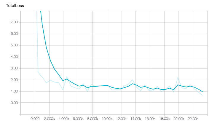
Total loss decreased pretty fast due to the pre-trained model.

Since I only had one class, it was enough to just look at total mAP (mean average precision):

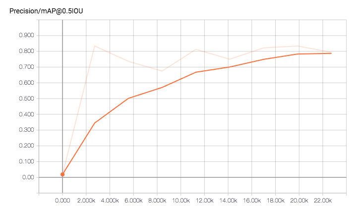
The mAP hit 0.8 at around 20k steps which is quite good.

And here is an example for the evaluation of one image while training the model:

The detected box around the Raccoon got much better over time.

  

---

 

Creating insanely fast image classifiers with MobileNet in TensorFlow 识别大马路

 

With that, let’s learn the following:

• What are MobileNets? 是什么
• How to build a custom dataset to train a MobileNet with TensorFlow 数据库
• How to train a MobileNet that’s pretrained on ImageNet with TensorFlow 训练
• How MobileNets perform against Inception V3
• How to use your retrained MobileNet to classify images

 

What are MobileNets?

MobileNets are a class of convolutional neural network designed by researches at Google. They are coined “mobile-first” in that they’re architected from the ground up to be resource-friendly and run quickly, right on your phone.

The main difference between the MobileNet architecture and a “traditional” CNN’s is instead of a single 3x3 convolution layer followed by batch norm and ReLU, MobileNets split the convolution into a 3x3 depthwise conv and a 1x1 pointwise conv. The details of why this is so significant can be found in the MobileNet paper, which I strongly encourage you to read.

So what’s the catch? Accuracy. MobileNets are not usually as accurate as the bigger, more resource-intensive networks we’ve come to know and love. But finding that resource/accuracy trade-off is where MobileNets really shine.

MobileNets surface two parameters that we can tune to fit the resource/accuracy trade-off of our exact problem: width multiplier and resolution multiplier. The width multiplier allows us to thin the network, while the resolution multiplier changes the input dimensions of the image, reducing the internal representation at every layer.

Google open-sourced the MobileNet architecture and released 16 ImageNet checkpoints, each corresponding to a different parameter configuration. This gives us an excellent starting point for training our own classifiers that are insanely small and insanely fast.

To learn more about how MobileNets work, read MobileNets: Efficient Convolutional Neural Networks for Mobile Vision Applications.

 

How to build your own dataset to train a MobileNet

Our challenge today is to build an image classifier that can detect if an image is a road or not a road. It’s like hot dog, not hot dog, but for roads.

Why road, not road? At Coastline, we’re developing safety features for your car with mobile apps that use computer vision. As with all vision problems, user privacy is critical. So one of the first checks we do when a user turns on the camera in our app is check if it sees a road. If it doesn’t, we turn off the camera. We want to be able to do this fast and at as little computational cost to the user as possible.

Since we’re tackling a custom problem, we need to start with creating our dataset. Our target is to collect 10,000 images, split roughly evenly 50/50 road/not road.

 

We’ll get data from a few different places:

• • 4,000 obviously road images sampled randomly from the Coastline driving dataset
  • 2,000 obviously not road images sampled randomly from the ImageNet dataset
  • 3,000 less obviously not road scenics sampled from the internet to make sure the classifier doesn’t just learn sky, not sky
  • 1,000 less obviously road scenics also sampled from the internet to make sure the classifier doesn’t recognize windshield reflections or other commonalities in the Coastline data

We’ll place each image into one of two folders, each representing the class of that image: road and not-road. That’s all we have to do to prepare our images for retraining!

However, while grabbing CC images from the internet is a great place to add diversity to your dataset, it comes with a drawback: the labels are noisy. For instance, an image found by searching “road landscape” could have a road front and center with a nice scene in the background, or it could be a mountain scene with a tiny road off in the distance.

 

How to retrain a MobileNet that’s pretrained on ImageNet 【train】

TensorFlow comes packaged with great tools that you can use to retrain MobileNets without having to actually write any code.

This stuff is fresh off the presses: Retraining support for MobileNet was added less than a week ago!

 

【关键是retrain.py的使用问题！】

Let’s retrain a small assortment and see how they perform. To kick off training, we’ll run the following command from the root of the TensorFlow repo:

python tensorflow/examples/image_retraining/retrain.py \ --image_dir               ~/ml/blogs/road-not-road/data/ \ --learning_rate           =0.0001 \ --testing_percentage      =20 \ --validation_percentage   =20 \ --train_batch_size        =32 \ --validation_batch_size   =-1 \ --flip_left_right True \ --random_scale            =30 \ --random_brightness       =30 \ --eval_step_interval      =100 \ --how_many_training_steps =600 \ --architecture mobilenet_1.0_224

 【1.0，224是mobileNet的两个参数】

 

可见，是训练top layer：

Simple transfer learning with Inception v3 or Mobilenet models.
With support for TensorBoard.
This example shows how to take a Inception v3 or Mobilenet model trained on ImageNet images, and train a new top layer that can recognize other classes of images.
The top layer receives as input a 2048-dimensional vector (1001-dimensional for Mobilenet) for each image. We train a softmax layer on top of this representation.

Assuming the softmax layer contains N labels, this corresponds to learning N + 2048*N (or 1001*N) model parameters corresponding to the learned biases and weights.
Here's an example, which assumes you have a folder containing class-named subfolders, each full of images for each label. The example folder flower_photos should have a structure like this:

~/flower_photos/daisy/photo1.jpg

~/flower_photos/daisy/photo2.jpg

...

 

Some other important parameters:

• • learning_rate: This is something you’ll want to play with. I found 0.0001 to work well.
  • testing and validation percentage: The script will split your data into train/val/test for you. It will use train to train, val to give performance updates every “eval_step_interval”, and test will run after “how_many_training_steps” to give you your final score.
  • validation_batch_size: Setting this to -1 tells the script to use all your data to validate on. When you don’t have a lot of data (like only 10,000 images), it’s a good idea to use -1 here to reduce variance between evaluation steps.

After retraining on several model architectures, let’s see how they compare.

 

Comparing MobileNet parameters and their performance against Inception   <---- 惊讶的性能

After just 600 steps on training Inception to get a baseline (by setting the — architecture flag to inception_v3), we hit 95.9%. Training took 18 minutes. (There is a lot of room for improvement here, but we don’t have all day!) The resulting checkpoint landed at 84mb. And doing a quick speed test by running 1,000 images through it shows it can classify images on an NVIDIA GeForce 960m GPU at ~19fps.

Aside: Why “only” 95.9% and not 100%? It seems like a pretty simple problem, right? Well, besides the ample tuning we could do to the training parameters (we actually achieved 98.9% with the same data using a different configuration in another go), it turns out the distinction between classes is a bit more subtle than it seems on the surface. Take these cases:

• • The image is a one-lane dirt road in the woods: Is it a road or a trail? I don’t even know.
  • It’s a landscape scenic with a road in the distance. Is it a picture or a road, or is there just a road in the picture? At what point does the scenic move classes?
  • It’s an artsy tilt-shift photo of a couple holding hands in the foreground and a time-lapsed street in the background. Road or not road? Flip a coin.

 

So, how do the MobileNets perform? Not surprisingly, not quite as well. However, the tradeoff benefit is astounding.

• • Using the biggest MobileNet (1.0, 224), we were able to achieve 95.5% accuracy with just 4 minutes of training. The resulting model size was just 17mb, and it can run on the same GPU at ~135fps.
  • How about the smallest MobileNet (0.24, 128), using quantized weights? Big accuracy tradeoff, achieving just 89.2%. But get this: 450 frames per second, and the model takes just 930kb of memory. That’s kilobytes!

  

Using your retrained MobileNet to classify images 【test】

Now that you have your MobileNet retrained on your custom dataset, it’s time to give it a try. Not surprisingly, TensorFlow comes with a script to do that, too.

python3 tensorflow/examples/label_image/label_image.py \ --graph=/tmp/mobilenet_0.50_192.pb \ --labels=/tmp/output_labels.txt \ --image=/home/harvitronix/ml/blogs/road-not-road/test-image.jpg \ --input_layer  =input \ --output_layer =final_result \ --input_mean   =128 \ --input_std    =128 \ --input_width  =192 \ --input_height =192

 

以上都是PC上的实验效果：400 frames per second on a laptop.

手机上的效果还需要进一步的实验.

 

 

Goals and Plan

Let’s set some constraints so we have something specific to shoot for. We’ll attempt to:

• • Retrain a MobileNet on a very small amount of purpose-built data
  • Achieve 95% classification accuracy on a hold out test set
  • Use less than 5% of a $300 device’s CPU while running inference

To do that, we’ll follow these steps:

1. 1. Generate a new training dataset 数据
   2. Train several MobileNet configurations to find the smallest net that will hit our accuracy target 尽可能小的网络
   3. Get benchmarks by running Inception V3 on Android 拿v3作为对比参照
   4. Update the TensorFlow Android example app to use our MobileNet model
   5. Try it in the wild
   6. Tune it to get below 5% CPU usage

 

Building the Dataset

In the previous post, we were classifying road/not road generally, so we pulled images from several sources. Now we’re going to drill down on the problem a bit more.

If you recall, the purpose for this project is for user privacy: At Coastline, we’re building driving safety features for mobile devices that make use of the camera.

So when someone turns on the app, we want to validate that what we’re looking at is a road. If we aren’t, we’ll disable recording.

So to build our training set, I’m going to walk around doing everyday things while recording video: Around my house, outside my car, inside my car fiddling with the radio, petting the cats, etc. This will be our “not road” training data.

With 3,000 examples from each set, we’re ready to train.

【总之要尽可能的丰富】

 

Training MobileNet on our custom dataset 【建模】

The next step is to see what sort of accuracy we can get from the different MobileNet configurations.

We’ll start with training the widest one: MoileNet 1.0 @ 128.

And because we’re going to put this on a mobile device, we’ll use [quantized weights], which will reduce the model memory footprint even further.

For the details on how to retrain MobileNet on your own data, be sure to check out my previous post.

From the root TensorFlow folder, we’ll run:

python tensorflow/examples/image_retraining/retrain.py \ --image_dir               ~/ml/blogs/road-not-road/data/ \ --learning_rate           =0.0005 \ --testing_percentage      =15 \ --validation_percentage   =15 \ --train_batch_size        =32 \ --validation_batch_size   =-1 \ --flip_left_right True \ --random_scale            =30 \ --random_brightness       =30 \ --eval_step_interval      =100 \ --how_many_training_steps =1000 \ --architecture            mobilenet_1.0_128_quantized

After 1,000 training steps, we achieve 99.7% accuracy on our hold out set. Wow! Apparently MobileNets are pretty good at classifying roads.

 

Here are a couple images it miss-classified:

Now let’s do the same thing, but with the smallest MobileNet: 0.25 @ 128, quantized.

After 1,000 training steps, we get to 92.6%. Doesn’t satisfy our accuracy target.

 

How about something a little wider, say 0.5?

95.0%! And the final model is just 1.6 MB. Looks like our money shot, if just barely. (It should be noted that this entire model is trained on just 10 minutes of video captured at 10fps. There is a lot of room for improvement by piling on the data.)

 

Let’s give it a quick try to make sure it’s working as expected:

python tensorflow/examples/label_image/label_image.py \ --graph           = /tmp/output_graph.pb \ --labels          = /tmp/output_labels.txt \ --image           = /home/harvitronix/ml/blogs/road-not-road/test-image.jpg \ --input_layer     = input \ --output_layer    = final_result \ --input_mean      = 128 \ --input_std       = 128 \ --input_width     = 128 \ --input_height    = 128 

And since our headline has the words “insanely fast” in it, how fast can we run this on an NVIDIA GeForce 960m GPU on our laptop? It runs through 1,000 images in just 3.36 seconds. That’s 297.6 frames per second!

 

Using our MobileNet model in an Android app 【实测】

Now that we have a model that’s tiny, fast and accurate enough for our use case, let’s load it up in an Android app so we can test it in the real world.

Don’t have a model trained yet? Download the model I trained on the data described above. It contains both the .pb and label files. Extract and follow the instructions below.

Sticking with our theme of using tools provided by TensorFlow (how awesome is that, btw?), we’ll make use of the Android example project to get this thing running in no time flat.

【不妨实践下】

 

Getting and building the project 【Or 自己亲自做下】

• Inception V3效果

If you haven’t already, go ahead and clone the TensorFlow repo:

git clone https://github.com/tensorflow/tensorflow.git --depth 1

You’ll find an Android project ready-made for doing this kind of task in the tesnorflow/examples/android folder.

应该是基于V3的分类器：

Open the folder in Android Studio, build it, load the APK on your phone, and you’ve got an image classifier that uses the Inception V3 model trained on ImageNet, ready to tell apart your cat from a platypus.

If you have trouble building the app, be sure to take a look at the instructions in the TensorFlow Android ReadMe. My biggest challenge was the NDK version. Downgrading to r12b solved my problems.

 

Inception speed benchmark

Since we’ve already got Inception running on the app, let’s take some measurements so we can compare it against our MobileNet.

The Inception model that comes with the example project is 53.9 mb. That’s versus our MobileNet that’s just 1.6 mb! It runs at about 240ms per inference, or 4 frames per second (fps). And it uses about 40% of the CPU.

Inception V3 running at 4fps.

Let’s try it at 1fps: 

Inception V3 running at 1fps.

Still up over 35%. Let’s hope our MobileNet can do better than that, or we’re not going to get anywhere near our goal of max 5% usage.

 

• MobileNet 效果

Now let’s make a couple minor changes to the Android project to use our custom MobileNet model.

First, copy your model and labels into the project’s assets folder. Mine were at /tmp/output_graph.pb and /tmp/output_labels.txt.

Next, open up ClassifierActivity, which can be found in:

tensorflow/examples/android/src/org/tensorflow/demo/ClassifierActivity.java

 

You’ll want to update the constants at the top of the file to define the settings for our new model. It looks like this when you first open it:

private static final int INPUT_SIZE     = 224; private static final int IMAGE_MEAN = 117; private static final float IMAGE_STD = 1; private static final String INPUT_NAME = "input"; private static final String OUTPUT_NAME = "output"; private static final String MODEL_FILE = "file:///android_asset/tensorflow_inception_graph.pb"; private static final String LABEL_FILE = "file:///android_asset/imagenet_comp_graph_label_strings.txt";

Change it to:

private static final int INPUT_SIZE     = 128; private static final int IMAGE_MEAN = 128; private static final float IMAGE_STD = 128; private static final String INPUT_NAME = "input"; private static final String OUTPUT_NAME = "final_result"; private static final String MODEL_FILE = "file:///android_asset/output_graph.pb"; private static final String LABEL_FILE = "file:///android_asset/output_labels.txt";

Hit run to build the project and load the APK on your device, and you’ve got your very own road / not road classifier!

 

竟然用的是小米手机测试：

On my Xiaomi Mi5, this thing flies. It does inference in about 55ms, which is 18 frames per second! On a $300 Xiaomi Mi5s!

 

It is quite CPU intensive, though, using 25–30% when running at full-throttle. Makes sense, since we’re running it as fast as it will go. 

MobileNEt CPU monitor, running at 18fps.

We want to get down to under 5%, which we’ll do by reducing the frequency at which it runs, since our use case doesn’t need to run inference continuously to achieve our privacy objective discussed above. Changing it to classify once every 18 frames (so once a second, roughly) brings the average usage down to about 5.5%! 

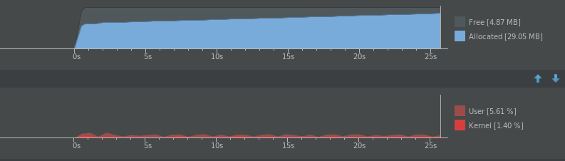
MobileNet running at 1fps.

So our MobileNet model is 1/30th as large as Inception. It runs more than 3x faster per frame. And it uses far fewer CPU resources.

【完胜！】